

Quantile Calibration#
Improve the reliability of probabilistic forecasts using isotonic and asymmetric conformal quantile calibration. A well-calibrated P10 quantile should exceed actual values roughly 10 % of the time — this tutorial shows how to measure and correct deviations.
What you’ll learn:
Measure quantile calibration with observed coverage
Add isotonic and asymmetric conformal calibration as postprocessing steps
Compare before/after calibration on real data
Note
This tutorial uses a small data slice for fast execution.
Key API references:
IsotonicQuantileCalibrator
· ConformalizedQuantileCalibrator
· ForecastingWorkflowConfig
Load data and train an uncalibrated model#
We start with the same GBLinear setup as the Forecasting Quickstart and
measure how well its predicted quantiles match observed coverage.
The ForecastingWorkflowConfig
defines the model architecture and quantile levels.
from datetime import datetime, timedelta

import pandas as pd
import plotly.graph_objects as go

from openstef_core.testing import load_liander_dataset
from openstef_core.types import LeadTime, Q
from openstef_models.presets import ForecastingWorkflowConfig, create_forecasting_workflow
from openstef_models.presets.forecasting_workflow import GBLinearForecaster

dataset = load_liander_dataset()

train_start = datetime.fromisoformat("2024-03-01T00:00:00Z")
train_end = train_start + timedelta(days=45)
cal_end = train_end + timedelta(days=4)
forecast_end = cal_end + timedelta(days=7)

train_dataset = dataset.filter_by_range(start=train_start, end=train_end)
predict_dataset = dataset.filter_by_range(
    start=cal_end - timedelta(days=14),
    end=forecast_end,
)

quantiles = [Q(0.1), Q(0.5), Q(0.9)]

config = ForecastingWorkflowConfig(
    model_id="uncalibrated_gblinear",
    model="gblinear",
    horizons=[LeadTime.from_string("PT36H")],
    quantiles=quantiles,
    target_column="load",
    temperature_column="temperature_2m",
    relative_humidity_column="relative_humidity_2m",
    wind_speed_column="wind_speed_10m",
    radiation_column="shortwave_radiation",
    pressure_column="surface_pressure",
    verbosity=0,
    mlflow_storage=None,
    gblinear_hyperparams=GBLinearForecaster.HyperParams(n_steps=50),
)

workflow_uncal = create_forecasting_workflow(config=config)
workflow_uncal.fit(train_dataset)
forecast_uncal = workflow_uncal.predict(predict_dataset, forecast_start=cal_end)

print(f"Forecast rows: {len(forecast_uncal.data)}")
Forecast rows: 672
Measure calibration quality#
For a perfectly calibrated forecast at quantile \(p\), the fraction of observations falling below the predicted value should equal \(p\). We compute the observed coverage for each quantile and compare it to the expected level.
actuals = predict_dataset.data["load"].loc[train_end:].reindex(forecast_uncal.data.index).dropna()
forecast_aligned = forecast_uncal.data.loc[actuals.index]

expected = [float(q) for q in quantiles]
observed_uncal = [float((actuals <= forecast_aligned[f"quantile_P{int(float(q) * 100)}"]).mean()) for q in quantiles]

calibration_df = pd.DataFrame(
    {
        "quantile": [f"P{int(float(q) * 100)}" for q in quantiles],
        "expected": expected,
        "observed": observed_uncal,
        "error": [o - e for o, e in zip(observed_uncal, expected, strict=True)],
    }
)
print("Calibration before isotonic correction:")
print(calibration_df.to_string(index=False))
Calibration before isotonic correction:
quantile  expected  observed     error
     P10       0.1  0.025298 -0.074702
     P50       0.5  0.099702 -0.400298
     P90       0.9  0.297619 -0.602381
Add isotonic and asymmetric conformal calibration#
IsotonicQuantileCalibrator learns a
monotonic mapping from predicted quantiles to observed quantile levels. It is
appended to the workflow’s postprocessing pipeline and fitted on training-set
predictions automatically.
ConformalizedQuantileCalibrator
instead applies asymmetric conformal corrections. It leaves
P50 unchanged by default and delegates quantile ordering to a downstream
QuantileSorter.
from openstef_models.transforms.postprocessing import IsotonicQuantileCalibrator

config_cal = config.model_copy(update={"model_id": "calibrated_gblinear"})
workflow_cal = create_forecasting_workflow(config=config_cal)

# Append isotonic calibration to the existing postprocessing pipeline
workflow_cal.model.postprocessing.transforms.append(
    IsotonicQuantileCalibrator(
        quantiles=quantiles,
        use_local_quantile_estimation=True,
    )
)

workflow_cal.fit(train_dataset)
forecast_cal = workflow_cal.predict(predict_dataset, forecast_start=cal_end)
Calibrate with the asymmetric conformal transform#
Split-conformal calibration requires a held-out calibration period that the forecaster was not trained on. We predict that period with the fitted workflow, attach the observed target, and fit the calibrator before applying it to the final holdout forecast.
from openstef_models.transforms.postprocessing import ConformalizedQuantileCalibrator

calibration_dataset = dataset.filter_by_range(
    start=train_end - timedelta(days=14),
    end=cal_end,
)
workflow_conformalized = create_forecasting_workflow(
    config=config.model_copy(update={"model_id": "conformalized_gblinear"})
)
workflow_conformalized.fit(train_dataset)
cal_forecast = workflow_conformalized.predict(calibration_dataset, forecast_start=train_end)
conformalized_calibrator = ConformalizedQuantileCalibrator(quantiles=quantiles)
conformalized_calibrator.fit(cal_forecast)
forecast_conformalized_raw = workflow_conformalized.predict(predict_dataset, forecast_start=cal_end)
forecast_conformalized = conformalized_calibrator.transform(forecast_conformalized_raw)
Compare calibration before and after#
The following table and plot compare the uncalibrated forecast with both postprocessing approaches on the same holdout rows.
Isotonic calibration#
Isotonic calibration learns a monotonic mapping for each quantile. The
observed (isotonic) and error (isotonic) columns show its effect.
Asymmetric conformal calibration#
The observed (conformalized) and error (conformalized) columns show
the effect of the asymmetric corrections.
forecast_cal_aligned = forecast_cal.data.loc[actuals.index]
forecast_conformalized_aligned = forecast_conformalized.data.loc[actuals.index]

observed_cal = [float((actuals <= forecast_cal_aligned[f"quantile_P{int(float(q) * 100)}"]).mean()) for q in quantiles]
observed_conformalized = [
    float((actuals <= forecast_conformalized_aligned[f"quantile_P{int(float(q) * 100)}"]).mean()) for q in quantiles
]

comparison_df = pd.DataFrame(
    {
        "quantile": [f"P{int(float(q) * 100)}" for q in quantiles],
        "expected": expected,
        "observed (before)": observed_uncal,
        "observed (isotonic)": observed_cal,
        "observed (conformalized)": observed_conformalized,
        "error (before)": [o - e for o, e in zip(observed_uncal, expected, strict=True)],
        "error (isotonic)": [o - e for o, e in zip(observed_cal, expected, strict=True)],
        "error (conformalized)": [o - e for o, e in zip(observed_conformalized, expected, strict=True)],
    }
)
print(comparison_df.to_string(index=False))
quantile  expected  observed (before)  observed (isotonic)  observed (conformalized)  error (before)  error (isotonic)  error (conformalized)
     P10       0.1           0.025298             0.081845                  0.105655       -0.074702         -0.018155               0.005655
     P50       0.5           0.099702             0.409226                  0.101190       -0.400298         -0.090774              -0.398810
     P90       0.9           0.297619             0.922619                  0.901786       -0.602381          0.022619               0.001786
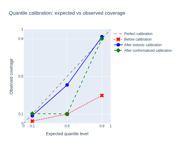
Points closer to the diagonal indicate better calibration. Isotonic regression learns a monotonic value mapping, while the conformalized calibrator applies asymmetric corrections. Compare both methods on a separate holdout period before selecting one for production. To measure calibration stability over longer time horizons, combine this with a Backtesting Quickstart.
Next steps#
Backtesting Quickstart — measure calibration consistency over realistic operational periods.
Ensemble Forecasting — apply calibration to ensemble models for combined accuracy and reliable uncertainty.