

Backtesting Quickstart#
Backtesting simulates how a forecasting model would have performed in a real operational setting. Unlike a simple train/test split, it respects temporal constraints: models are retrained on a schedule and predictions use only data that would have been available at prediction time.
What you will learn:
How to set up a backtesting pipeline with
BacktestPipelineHow to configure prediction and retraining schedules
How to evaluate backtest results with standardized metrics
Note
This tutorial shows the low-level backtesting API step by step.
For production use, the benchmark framework (openstef_beam.benchmarking)
wraps all of this into a single pipeline call — see
examples/benchmarks/ for ready-to-run examples.
Key API references:
BacktestPipeline
· BacktestConfig
· BacktestForecasterConfig
· EvaluationConfig
How backtesting works#
A backtesting pipeline replays history as if it were happening in real-time:
Event generation — the pipeline creates a schedule of prediction and retraining events based on configured intervals.
Training — at each retraining event, the model is fitted on all data available up to that point (no lookahead).
Prediction — at each prediction event, the model generates a forecast using only data published before that moment.
Collection — all forecasts are gathered into a single dataset for evaluation against ground truth.
Load the versioned dataset#
Backtesting requires versioned data — each data point carries an
available_at timestamp indicating when it became known. This prevents
the model from accidentally using future information.
VersionedTimeSeriesDataset
provides this out of the box.
from pathlib import Path

from openstef_core.datasets import VersionedTimeSeriesDataset
from openstef_core.testing import load_liander_dataset

# Download the dataset from HuggingFace (cached after first run)
data_dir = Path("liander_dataset")
load_liander_dataset(local_dir=data_dir)

# Ground truth: actual load measurements
ground_truth = VersionedTimeSeriesDataset.read_parquet(
    data_dir / "load_measurements" / "mv_feeder" / "OS Gorredijk.parquet"
)

# Predictors: versioned weather forecasts (available_at < forecast time)
predictors = VersionedTimeSeriesDataset.read_parquet(
    data_dir / "weather_forecasts_versioned" / "mv_feeder" / "OS Gorredijk.parquet"
)

print(f"Ground truth: {len(ground_truth.index):,} timestamps, {len(ground_truth.feature_names)} features")
print(f"Predictors:   {len(predictors.index):,} timestamps, {len(predictors.feature_names)} features")
Ground truth: 35,136 timestamps, 1 features
Predictors:   35,229 timestamps, 11 features
Configure the forecaster#
We wrap a standard ForecastingWorkflowConfig in an
OpenSTEF4BacktestForecaster which implements the backtesting interface
(fit/predict with temporal constraints).
from datetime import timedelta

from openstef_beam.backtesting.backtest_forecaster import BacktestForecasterConfig
from openstef_beam.benchmarking.baselines.openstef4 import OpenSTEF4BacktestForecaster
from openstef_core.types import LeadTime, Q
from openstef_models.presets import ForecastingWorkflowConfig, create_forecasting_workflow

workflow_config = ForecastingWorkflowConfig(
    model_id="backtest_demo",
    model="xgboost",
    horizons=[LeadTime.from_string("PT48H")],
    quantiles=[Q(0.5), Q(0.1), Q(0.9)],
    target_column="load",
    temperature_column="temperature_2m",
    relative_humidity_column="relative_humidity_2m",
    wind_speed_column="wind_speed_10m",
    radiation_column="shortwave_radiation",
    pressure_column="surface_pressure",
    mlflow_storage=None,
    verbosity=0,
)

backtest_forecaster_config = BacktestForecasterConfig(
    requires_training=True,
    predict_length=timedelta(hours=48),
    predict_min_length=timedelta(minutes=15),
    predict_context_length=timedelta(days=14),
    predict_context_min_coverage=0.5,
    training_context_length=timedelta(days=90),
    training_context_min_coverage=0.5,
)

workflow = create_forecasting_workflow(workflow_config)
forecaster = OpenSTEF4BacktestForecaster(
    config=backtest_forecaster_config,
    workflow_template=workflow,
    cache_dir=Path("cache/backtest_demo"),
)

print(f"Model:            {workflow_config.model}")
print(f"Training window:  {backtest_forecaster_config.training_context_length}")
print(f"Predict horizon:  {backtest_forecaster_config.predict_length}")
Model:            xgboost
Training window:  90 days, 0:00:00
Predict horizon:  2 days, 0:00:00
Run the backtest#
We configure the pipeline to predict every 6 hours and retrain weekly. The backtest covers a short 5-day window for fast execution.
from datetime import datetime

from openstef_beam.backtesting import BacktestConfig, BacktestPipeline

backtest_config = BacktestConfig(
    prediction_sample_interval=timedelta(minutes=15),
    predict_interval=timedelta(hours=6),
    train_interval=timedelta(days=7),
)

pipeline = BacktestPipeline(config=backtest_config, forecaster=forecaster)

# Short evaluation window: 5 days starting well into the dataset
backtest_start = datetime.fromisoformat("2024-05-01T00:00:00Z")
backtest_end = datetime.fromisoformat("2024-05-06T00:00:00Z")

predictions = pipeline.run(
    ground_truth=ground_truth,
    predictors=predictors,
    start=backtest_start,
    end=backtest_end,
)

print(f"Predictions generated: {predictions.data.shape[0]:,} rows")
print(f"Time range: {predictions.data.index.min()} to {predictions.data.index.max()}")
Predictions generated: 3,840 rows
Time range: 2024-05-01 00:00:00+00:00 to 2024-05-07 17:45:00+00:00
Evaluate the results#
The EvaluationPipeline computes metrics over configurable time windows.
It filters predictions by lead time to produce meaningful comparisons
(e.g., day-ahead forecasts only).
We use rMAE (relative Mean Absolute Error) and rCRPS (relative Continuous Ranked Probability Score) — both normalized by mean absolute actuals. See the full list of available metrics. If your scores are suboptimal, Hyperparameter Tuning with Optuna shows how to optimize model parameters before re-running the backtest.
from openstef_beam.evaluation import EvaluationConfig, EvaluationPipeline, Window
from openstef_beam.evaluation.metric_providers import RCRPSProvider, RMAEProvider

evaluation_config = EvaluationConfig(
    windows=[Window(lag=timedelta(hours=0), size=timedelta(days=5))],
    lead_times=[],  # Only use available_at filtering (day-ahead)
)

eval_pipeline = EvaluationPipeline(
    config=evaluation_config,
    quantiles=workflow_config.quantiles,
    window_metric_providers=[
        RMAEProvider(quantiles=[Q(0.5)]),
        RCRPSProvider(),
    ],
    global_metric_providers=[
        RMAEProvider(quantiles=[Q(0.5)]),
        RCRPSProvider(),
    ],
)

report = eval_pipeline.run(
    predictions=predictions,
    ground_truth=ground_truth,
    target_column="load",
)

print("Backtest evaluation metrics (day-ahead):")
for subset_report in report.subset_reports:
    print(f"\n  Lead-time filter: {subset_report.filtering}")
    for metric in subset_report.metrics:
        df = metric.to_dataframe()
        print(f"  Window: {metric.window}")
        print(df.to_string(index=False))
Backtest evaluation metrics (day-ahead):

  Lead-time filter: D-1T0600
  Window: (lag=PT0S,size=P5D,stride=P1D)
quantile     rMAE    rCRPS
     0.5 0.087587      NaN
  global      NaN 0.065455
  Window: global
quantile     rMAE  observed_probability    rCRPS
     0.5 0.087364              0.557971      NaN
  global      NaN                   NaN 0.064408
     0.1      NaN              0.369565      NaN
     0.9      NaN              0.768116      NaN
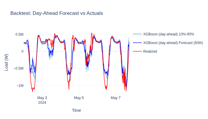
Visualize predictions vs actuals#
The evaluation report contains a properly filtered ForecastDataset for
each lead-time subset. We use this directly for visualization — it
shows only day-ahead predictions aligned with their corresponding actuals.
The easy way: benchmark framework#
The code above demonstrates each backtesting step explicitly. In practice, the benchmark framework handles all of this (data loading, target management, evaluation, analysis) in a single pipeline:
from openstef_beam.benchmarking.benchmarks.liander2024 import (
    create_liander2024_benchmark_runner,
)
from openstef_beam.benchmarking.baselines.openstef4 import (
    create_openstef4_preset_backtest_forecaster,
)

runner = create_liander2024_benchmark_runner()
forecaster_factory = create_openstef4_preset_backtest_forecaster(workflow_config)
runner.run(forecaster_factory, run_name="my_experiment")
The benchmark runner automatically:
Downloads and manages the dataset
Iterates over all targets (feeders, transformers, solar parks, etc.)
Runs backtests with standardized configuration
Computes metrics and generates analysis visualizations
See examples/benchmarks/ for complete benchmark scripts that will be
converted to Jupytext tutorials in a future update.
Next steps#
Hyperparameter Tuning with Optuna — optimize model parameters, then re-run the backtest to measure improvement.
Ensemble Forecasting — backtest an ensemble of diverse models.