Feature Engineering for Energy Forecasting

Energy load follows strong daily and weekly patterns driven by human behaviour, weather, and calendar effects. Raw time series alone don’t expose these patterns to a model — feature engineering makes them explicit.

OpenSTEF provides a library of transforms organized into five groups:

Group	Transforms	Purpose
Time Domain	CyclicFeaturesAdder, DatetimeFeaturesAdder, HolidayFeatureAdder, LagsAdder, RollingAggregatesAdder, VersionedLagsAdder	Encode temporal patterns
Weather Domain	DaylightFeatureAdder, AtmosphereDerivedFeaturesAdder, RadiationDerivedFeaturesAdder	Derive meteorological features
Energy Domain	WindPowerFeatureAdder	Power curve estimation
General	Imputer, Scaler, OutlierHandler, SampleWeighter, Selector, Shifter, DimensionalityReducer, EmptyFeatureRemover, Flagger, NaNDropper	Data cleaning & normalization
Validation	CompletenessChecker, FlatlineChecker, InputConsistencyChecker	Data quality gates
Postprocessing	ConfidenceIntervalApplicator, IsotonicQuantileCalibrator, QuantileSorter	Forecast output refinement

This tutorial demonstrates each group with real data, explains why each transform matters for energy forecasting, and shows how to build your own.

See also

• Building a Custom Pipeline — full end-to-end custom model assembly

• Forecasting Quickstart — standard approach using presets

• Quantile Calibration — deep-dive into postprocessing calibration

Load sample data

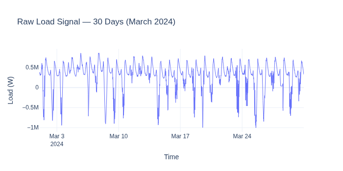
We use 30 days of real Dutch MV-feeder load data from March 2024. This period includes the spring equinox (rapidly changing daylight hours) and Easter (March 29-31), making it ideal for demonstrating calendar and daylight features.

from datetime import datetime, timedelta

import numpy as np
import pandas as pd
import plotly.graph_objects as go
from plotly.subplots import make_subplots

from openstef_core.datasets import TimeSeriesDataset
from openstef_core.testing import load_liander_dataset
from openstef_core.types import LeadTime

LOAD_LABEL = "Load (W)"
MODE_LINES_MARKERS = "lines+markers"

dataset = load_liander_dataset()

# March 2024: spring equinox + Easter
start = datetime.fromisoformat("2024-03-01T00:00:00Z")
end = start + timedelta(days=30)
sample = dataset.filter_by_range(start=start, end=end)

print(f"Dataset: {sample.data.shape[0]:,} rows x {sample.data.shape[1]} columns")
print(f"Period: {sample.data.index[0]} → {sample.data.index[-1]}")
print(f"Sample interval: {sample.sample_interval}")

Dataset: 2,880 rows x 28 columns
Period: 2024-03-01 00:00:00+00:00 → 2024-03-30 23:45:00+00:00
Sample interval: 0:15:00

Show code cell source

Hide code cell source

fig = go.Figure()
fig.add_trace(
    go.Scatter(
        x=sample.data.index,
        y=sample.data["load"],
        mode="lines",
        name=LOAD_LABEL,
        line={"width": 1},
    )
)
fig.update_layout(
    title="Raw Load Signal — 30 Days (March 2024)",
    xaxis_title="Time",
    yaxis_title=LOAD_LABEL,
    height=350,
    template="plotly_white",
)
fig.show()

---

1. Time Domain Transforms

These transforms encode temporal patterns that drive energy consumption.

CyclicFeaturesAdder

What: Encodes hour-of-day, day-of-week, month, and season as sine/cosine pairs.

Why for energy forecasting: Energy demand has strong 24-hour and 7-day periodicity. Sine/cosine encoding makes the periodicity smooth and continuous — hour 23 is naturally close to hour 0. This helps both tree-based and linear models capture daily patterns with fewer parameters.

from openstef_models.transforms.time_domain import CyclicFeaturesAdder

cyclic = CyclicFeaturesAdder()
result = cyclic.transform(sample)

cyclic_cols = cyclic.features_added()
print(f"Added {len(cyclic_cols)} columns: {cyclic_cols}")

Added 8 columns: ['time_of_day_sine', 'season_sine', 'day_of_week_sine', 'month_sine', 'time_of_day_cosine', 'season_cosine', 'day_of_week_cosine', 'month_cosine']

Show code cell source

Hide code cell source

# Plot 3 days: load pattern aligned with time-of-day encoding
three_days = result.data.iloc[:288]  # 3 days x 96 intervals

fig = make_subplots(
    rows=2,
    cols=1,
    shared_xaxes=True,
    vertical_spacing=0.08,
    subplot_titles=("Load Pattern (3 days)", "Time-of-Day Cyclic Encoding"),
)
fig.add_trace(
    go.Scatter(x=three_days.index, y=three_days["load"], mode="lines", name="Load", line={"width": 1.5}), row=1, col=1
)

for col in [c for c in cyclic_cols if "time_of_day" in c]:
    fig.add_trace(
        go.Scatter(x=three_days.index, y=three_days[col], mode="lines", name=col, line={"width": 1.5}), row=2, col=1
    )

fig.update_layout(height=450, template="plotly_white", title="Cyclic Features Follow the Daily Load Pattern")
fig.show()

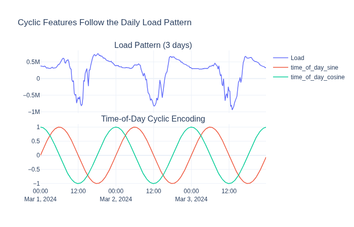
The sine/cosine curves align with the load’s daily rhythm — they peak and trough in sync with demand, giving the model a smooth “where in the day” signal.

HolidayFeatureAdder

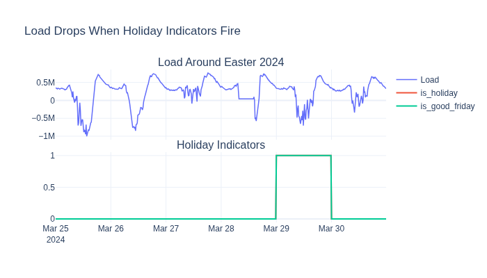
What: Adds binary flags for national holidays, school holidays, and bridge days.

Why for energy forecasting: On public holidays, industrial and commercial load disappears - demand can drop 20-40% below a normal weekday. Without explicit holiday features, the model would treat Good Friday as a regular Friday and overpredict.

from openstef_models.transforms.time_domain import HolidayFeatureAdder

holidays = HolidayFeatureAdder(country_code="NL")
result = holidays.transform(sample)

holiday_cols = holidays.features_added()
print(f"Added {len(holiday_cols)} columns: {holiday_cols}")

Added 12 columns: ['is_holiday', 'is_ascension_day', 'is_christmas_day', 'is_easter_monday', 'is_easter_sunday', 'is_good_friday', 'is_king_s_day', 'is_liberation_day', 'is_new_year_s_day', 'is_second_day_of_christmas', 'is_whit_monday', 'is_whit_sunday']

Show code cell source

Hide code cell source

# Show Easter weekend load drop with holiday indicators
easter_start = datetime.fromisoformat("2024-03-25T00:00:00Z")
easter_end = datetime.fromisoformat("2024-04-01T00:00:00Z")
easter_window = result.data.loc[easter_start:easter_end]

fig = make_subplots(
    rows=2,
    cols=1,
    shared_xaxes=True,
    vertical_spacing=0.08,
    subplot_titles=("Load Around Easter 2024", "Holiday Indicators"),
)
fig.add_trace(
    go.Scatter(x=easter_window.index, y=easter_window["load"], mode="lines", name="Load", line={"width": 1.5}),
    row=1,
    col=1,
)
for col in holiday_cols:
    if easter_window[col].any():
        fig.add_trace(
            go.Scatter(x=easter_window.index, y=easter_window[col], mode="lines", name=col, line={"width": 2}),
            row=2,
            col=1,
        )
fig.update_layout(height=400, template="plotly_white", title="Load Drops When Holiday Indicators Fire")
fig.show()

LagsAdder

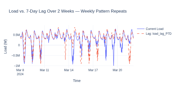
What: Creates time-shifted copies of the target column (e.g., “load 7 days ago”).

Why for energy forecasting: Energy demand is highly auto-correlated — last Monday’s load is the best predictor of this Monday’s load. The key constraint: lags must respect the forecast horizon. If you’re forecasting 36 hours ahead, you can’t use data from 24 hours ago. OpenSTEF’s LagsAdder automatically selects valid lags for each horizon.

from openstef_models.transforms.time_domain.lags_adder import LagsAdder

horizons = [LeadTime.from_string("PT36H")]

lags = LagsAdder(
    history_available=timedelta(days=14),
    horizons=horizons,
    add_trivial_lags=False,
    target_column="load",
    custom_lags=[timedelta(days=7)],
    lag_fallback_offset=timedelta(days=7),
)
result = lags.transform(sample)

lag_cols = lags.features_added()
print(f"Added {len(lag_cols)} lag columns: {lag_cols[:5]}")

Added 1 lag columns: ['load_lag_P7D']

Show code cell source

Hide code cell source

# Plot load vs its 7-day lag over 2 weeks
two_weeks = result.data.iloc[672:2016]
lag_7d_col = [c for c in lag_cols if "7 day" in c.lower() or "168" in c]
target_col = lag_7d_col[0] if lag_7d_col else lag_cols[0]

fig = go.Figure()
fig.add_trace(
    go.Scatter(x=two_weeks.index, y=two_weeks["load"], mode="lines", name="Current Load", line={"width": 1.5})
)
fig.add_trace(
    go.Scatter(
        x=two_weeks.index,
        y=two_weeks[target_col],
        mode="lines",
        name=f"Lag: {target_col}",
        line={"width": 1.5, "dash": "dash"},
    )
)
fig.update_layout(
    title="Load vs. 7-Day Lag Over 2 Weeks — Weekly Pattern Repeats",
    xaxis_title="Time",
    yaxis_title=LOAD_LABEL,
    height=350,
    template="plotly_white",
)
fig.show()

RollingAggregatesAdder

What: Computes rolling statistics (mean, median, min, max) over a configurable window.

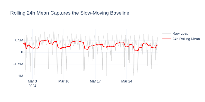
Why for energy forecasting: A 24-hour rolling mean captures the slow-moving “baseline demand” level, filtering out intra-day noise. This helps the model detect gradual shifts (e.g., temperature-driven HVAC ramp-ups).

from openstef_models.transforms.time_domain import RollingAggregatesAdder

rolling = RollingAggregatesAdder(
    feature="load",
    rolling_window_size=timedelta(hours=24),
    aggregation_functions=["mean", "max"],
    horizons=horizons,
)
rolling.fit(sample)
result = rolling.transform(sample)

rolling_cols = rolling.features_added()
print(f"Added: {rolling_cols}")

Added: ['rolling_mean_load_P1D', 'rolling_max_load_P1D']

Show code cell source

Hide code cell source

fig = go.Figure()
fig.add_trace(
    go.Scatter(
        x=result.data.index,
        y=result.data["load"],
        mode="lines",
        name="Raw Load",
        line={"width": 0.8, "color": "lightgray"},
    )
)
mean_col = next(c for c in rolling_cols if "mean" in c)
fig.add_trace(
    go.Scatter(
        x=result.data.index,
        y=result.data[mean_col],
        mode="lines",
        name="24h Rolling Mean",
        line={"width": 2, "color": "red"},
    )
)
fig.update_layout(title="Rolling 24h Mean Captures the Slow-Moving Baseline", height=350, template="plotly_white")
fig.show()

DatetimeFeaturesAdder

What: Extracts integer components (hour, day-of-week, month, etc.).

Why for energy forecasting: Datetime integers give tree models sharp split boundaries — e.g., “if hour >= 17 and hour <= 20 → evening peak.” Highly effective for XGBoost/LightGBM.

from openstef_models.transforms.time_domain import DatetimeFeaturesAdder

dt_features = DatetimeFeaturesAdder()
result = dt_features.transform(sample)

dt_cols = dt_features.features_added()
print(f"Added {len(dt_cols)} columns: {dt_cols}")
result.data[dt_cols].head(8)

Added 5 columns: ['is_week_day', 'is_weekend_day', 'is_sunday', 'month_of_year', 'quarter_of_year']

	is_week_day	is_weekend_day	is_sunday	month_of_year	quarter_of_year
timestamp
2024-03-01 00:00:00+00:00	1	0	0	3	1
2024-03-01 00:15:00+00:00	1	0	0	3	1
2024-03-01 00:30:00+00:00	1	0	0	3	1
2024-03-01 00:45:00+00:00	1	0	0	3	1
2024-03-01 01:00:00+00:00	1	0	0	3	1
2024-03-01 01:15:00+00:00	1	0	0	3	1
2024-03-01 01:30:00+00:00	1	0	0	3	1
2024-03-01 01:45:00+00:00	1	0	0	3	1

VersionedLagsAdder

What: Adds lags from a VersionedTimeSeriesDataset — data where each row has an available_at timestamp indicating when that observation became known.

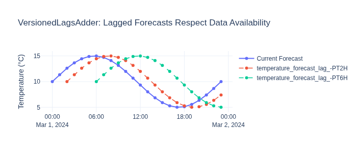
Why for energy forecasting: Weather forecasts are versioned: the forecast for Monday issued on Saturday differs from the one issued on Sunday. Standard lags ignore this — VersionedLagsAdder correctly uses only data that was actually available at prediction time, preventing data leakage.

from openstef_core.datasets import VersionedTimeSeriesDataset
from openstef_models.transforms.time_domain.versioned_lags_adder import VersionedLagsAdder

# Synthetic example: hourly temperature forecasts with availability tracking
index = pd.date_range("2024-03-01", periods=24, freq="1h", tz="UTC")
synth_data = pd.DataFrame(
    {
        "temperature_forecast": np.sin(np.linspace(0, 2 * np.pi, 24)) * 5 + 10,
        "available_at": index - pd.Timedelta(hours=6),  # available 6h before valid time
    },
    index=index,
)

versioned_ds = VersionedTimeSeriesDataset.from_dataframe(synth_data, timedelta(hours=1))

versioned_lags = VersionedLagsAdder(
    feature="temperature_forecast",
    lags=[timedelta(hours=-2), timedelta(hours=-6)],
)
result_v = versioned_lags.transform(versioned_ds)
snapshot = result_v.select_version()

lag_features = [c for c in snapshot.feature_names if "lag" in c]
print(f"Added lag features: {lag_features}")

Added lag features: ['temperature_forecast_lag_-PT2H', 'temperature_forecast_lag_-PT6H']

Show code cell source

Hide code cell source

fig = go.Figure()
fig.add_trace(
    go.Scatter(
        x=snapshot.data.index,
        y=snapshot.data["temperature_forecast"],
        mode=MODE_LINES_MARKERS,
        name="Current Forecast",
        line={"width": 2},
    )
)
for col in lag_features:
    fig.add_trace(
        go.Scatter(
            x=snapshot.data.index,
            y=snapshot.data[col],
            mode=MODE_LINES_MARKERS,
            name=col,
            line={"width": 1.5, "dash": "dash"},
        )
    )
fig.update_layout(
    title="VersionedLagsAdder: Lagged Forecasts Respect Data Availability",
    yaxis_title="Temperature (°C)",
    height=300,
    template="plotly_white",
)
fig.show()

---

2. Weather Domain Transforms

DaylightFeatureAdder

What: Computes sunrise, sunset, and daylight duration from coordinates.

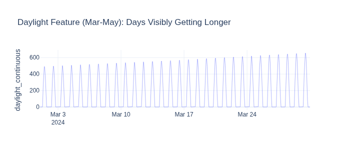
Why for energy forecasting: Daylight drives lighting demand and PV output. In spring, daylight changes ~3 min/day — a meaningful trend even within a month.

from openstef_models.transforms.weather_domain import DaylightFeatureAdder

daylight = DaylightFeatureAdder(coordinate=(52.0, 5.9))
result = daylight.transform(sample)

daylight_cols = daylight.features_added()
print(f"Added: {daylight_cols}")

Added: ['daylight_continuous']

Show code cell source

Hide code cell source

# Show the raw daylight feature over the full 3-month period
# The expanding bright periods from March→May show lengthening days
dl_col = daylight_cols[0]
fig = go.Figure()
fig.add_trace(go.Scatter(x=result.data.index, y=result.data[dl_col], mode="lines", name=dl_col, line={"width": 0.5}))
fig.update_layout(
    title="Daylight Feature (Mar-May): Days Visibly Getting Longer",
    yaxis_title=dl_col,
    height=300,
    template="plotly_white",
)
fig.show()

AtmosphereDerivedFeaturesAdder

What: Computes dewpoint, vapour pressure, and air density from temperature, pressure, and humidity.

Why for energy forecasting:

• Dewpoint → discomfort threshold → HVAC demand

• Air density → affects wind turbine output

• Vapour pressure → humidity signal for HVAC & PV efficiency

from openstef_models.transforms.weather_domain import AtmosphereDerivedFeaturesAdder

atmosphere = AtmosphereDerivedFeaturesAdder(
    included_features=["dewpoint", "air_density", "vapour_pressure"],
    temperature_column="temperature_2m",
    pressure_column="surface_pressure",
    relative_humidity_column="relative_humidity_2m",
)
result = atmosphere.transform(sample)

atmo_cols = atmosphere.features_added()
print(f"Added: {atmo_cols}")
result.data[atmo_cols].describe().loc[["mean", "std", "min", "max"]]

Added: ['dewpoint', 'air_density', 'vapour_pressure']

	dewpoint	air_density	vapour_pressure
mean	4.910169	1.244802	88125.625000
std	2.750122	0.020315	16598.488281
min	-2.756500	1.193168	49929.972656
max	11.743501	1.306328	137914.062500

RadiationDerivedFeaturesAdder

What: Computes Direct Normal Irradiance (DNI) and Global Tilted Irradiance (GTI) from horizontal radiation using solar geometry.

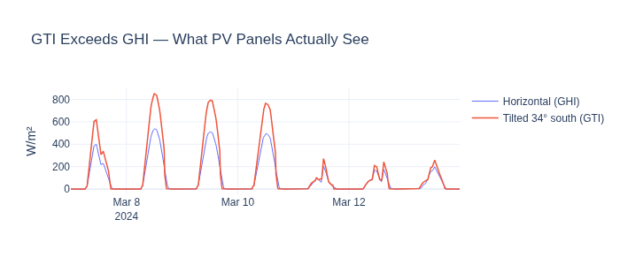
Why for energy forecasting: PV panels are tilted, not horizontal. GTI on a 34° south-facing panel is what actually drives generation — 20-40% higher than horizontal in winter.

from pydantic_extra_types.coordinate import Coordinate, Latitude, Longitude

from openstef_models.transforms.weather_domain import RadiationDerivedFeaturesAdder

radiation = RadiationDerivedFeaturesAdder(
    coordinate=Coordinate(latitude=Latitude(52.0), longitude=Longitude(5.9)),
    included_features=["dni", "gti"],
    surface_tilt=34.0,
    surface_azimuth=180.0,
    radiation_column="shortwave_radiation",
)
result = radiation.transform(sample)

rad_cols = radiation.features_added()
print(f"Added: {rad_cols}")

Added: ['dni', 'gti']

Show code cell source

Hide code cell source

sunny_week = result.data.iloc[576:1248]
fig = go.Figure()
fig.add_trace(
    go.Scatter(
        x=sunny_week.index,
        y=sunny_week["shortwave_radiation"],
        mode="lines",
        name="Horizontal (GHI)",
        line={"width": 1},
    )
)
if "gti" in rad_cols:
    fig.add_trace(
        go.Scatter(
            x=sunny_week.index, y=sunny_week["gti"], mode="lines", name="Tilted 34° south (GTI)", line={"width": 1.5}
        )
    )
fig.update_layout(
    title="GTI Exceeds GHI — What PV Panels Actually See", yaxis_title="W/m²", height=300, template="plotly_white"
)
fig.show()

---

3. Energy Domain Transforms

WindPowerFeatureAdder

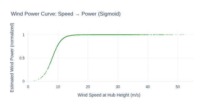
What: Extrapolates wind speed to hub height, then estimates power via a sigmoid power curve.

Why for energy forecasting: Wind speed at 10m doesn’t map linearly to turbine output. The relationship is a sigmoid (cut-in → rated → cut-out). This transform encodes that physics directly.

from openstef_models.transforms.energy_domain import WindPowerFeatureAdder

wind = WindPowerFeatureAdder(
    windspeed_reference_column="wind_speed_10m",
    reference_height=10.0,
    hub_height=100.0,
)
result = wind.transform(sample)

wind_cols = wind.features_added()
print(f"Added: {wind_cols}")

Added: ['wind_power']

Show code cell source

Hide code cell source

# Power curve: wind speed vs estimated power (non-linear relationship)
fig = go.Figure()
fig.add_trace(
    go.Scattergl(
        x=result.data["windspeed_hub_height"],
        y=result.data["wind_power"],
        mode="markers",
        name="Power curve",
        marker={"size": 2, "opacity": 0.5, "color": "green"},
    )
)
fig.update_layout(
    title="Wind Power Curve: Speed → Power (Sigmoid)",
    xaxis_title="Wind Speed at Hub Height (m/s)",
    yaxis_title="Estimated Wind Power (normalized)",
    height=350,
    template="plotly_white",
)
fig.show()

---

4. General Transforms (Data Cleaning & Preparation)

Imputer

What: Fills missing values (mean, median, forward-fill, etc.).

Why: Sensor failures create gaps. Models can’t train on NaN. The Imputer fills feature gaps while preserving the target column unchanged.

from openstef_models.transforms.general import Imputer
from openstef_models.utils.feature_selection import Exclude

imputer = Imputer(selection=Exclude("load"), imputation_strategy="mean")

# Simulate 2% missing data
noisy = sample.data.copy()
rng = np.random.default_rng(42)
mask = rng.random(noisy.shape) < 0.02
noisy[mask] = np.nan
noisy_ds = TimeSeriesDataset(data=noisy, sample_interval=sample.sample_interval)

result = imputer.fit_transform(noisy_ds)
print("NaN count per column:")
nan_comparison = pd.DataFrame({"before": noisy_ds.data.isna().sum(), "after": result.data.isna().sum()})
print(nan_comparison[nan_comparison["before"] > 0].to_string())

NaN count per column:
                          before  after
load                          53     53
temperature_2m                54      0
relative_humidity_2m          59      0
surface_pressure              49      0
cloud_cover                   37      0
wind_speed_10m                61      0
wind_speed_80m                52      0
wind_direction_10m            51      0
shortwave_radiation           63      0
direct_radiation              55      0
diffuse_radiation             45      0
direct_normal_irradiance      48      0
EPEX_NL                       69      0
E1A_AZI_A                     59      0
E1A_AMI_A                     61      0
E1B_AZI_A                     53      0
E1B_AMI_A                     62      0
E1C_AZI_A                     71      0
E1C_AMI_A                     55      0
E2A_AZI_A                     70      0
E2A_AMI_A                     53      0
E2B_AZI_A                     58      0
E2B_AMI_A                     58      0
E3A_A                         54      0
E3B_A                         68      1
E3C_A                         60      0
E3D_A                         47      0
E4A_A                         64      0

Scaler

What: Standardizes features to zero mean / unit variance.

Why: Features on different scales (temperature 0-16 °C vs radiation 0-633 W/m²) need normalization for neural networks and fair regularization.

from openstef_models.transforms.general import Scaler

scaler = Scaler(selection=Exclude("load"), method="standard")
result = scaler.fit_transform(sample)

weather_cols = ["temperature_2m", "shortwave_radiation", "wind_speed_10m"]
print("Before scaling (mean, std):")
print(sample.data[weather_cols].agg(["mean", "std"]).round(2).to_string())
print("\nAfter scaling (mean ≈ 0, std ≈ 1):")
print(result.data[weather_cols].agg(["mean", "std"]).round(2).to_string())

Before scaling (mean, std):
      temperature_2m  shortwave_radiation  wind_speed_10m
mean            7.87            96.449997           15.75
std             2.91           141.240005            6.43

After scaling (mean ≈ 0, std ≈ 1):
      temperature_2m  shortwave_radiation  wind_speed_10m
mean             0.0                 -0.0             0.0
std              1.0                  1.0             1.0

OutlierHandler

What: Learns feature bounds during training; clips or NaN-masks outliers.

Why: Sensor glitches produce impossible values (temperature 100°C). Outliers distort tree splits and scaling. This enforces plausible ranges.

from openstef_models.transforms.general import OutlierHandler
from openstef_models.utils.feature_selection import Include

outlier = OutlierHandler(
    selection=Include("temperature_2m", "wind_speed_10m"),
    mode="standard",
    n_std=3.0,
    outlier_action="clip",
)
outlier.fit(sample)

# Inject outliers
outlier_data = sample.data.copy()
outlier_data.iloc[100, outlier_data.columns.get_loc("temperature_2m")] = 50.0
outlier_data.iloc[200, outlier_data.columns.get_loc("wind_speed_10m")] = 100.0
outlier_ds = TimeSeriesDataset(data=outlier_data, sample_interval=sample.sample_interval)

result = outlier.transform(outlier_ds)
print(f"Temperature 50°C → clipped to {result.data['temperature_2m'].iloc[100]:.1f}°C")
print(f"Wind speed 100 m/s → clipped to {result.data['wind_speed_10m'].iloc[200]:.1f} m/s")

Temperature 50°C → clipped to 16.6°C
Wind speed 100 m/s → clipped to 35.1 m/s

SampleWeighter

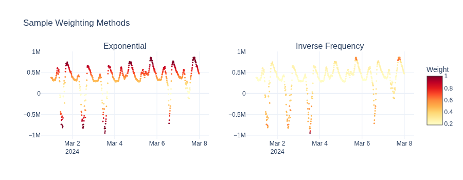
What: Assigns higher weights to peak-load samples during training.

Why: Peak load forecast errors are costlier (grid congestion, reserve activation). Weighting peaks higher makes the model pay more attention to the periods that matter most operationally.

from openstef_models.transforms.general import SampleWeighter
from openstef_models.transforms.general.sample_weighter import SampleWeightConfig

# Compare two weighting methods
weighter_exp = SampleWeighter(config=SampleWeightConfig(method="exponential"))
weighter_inv = SampleWeighter(config=SampleWeightConfig(method="inverse_frequency"))

result_exp = weighter_exp.fit_transform(sample)
result_inv = weighter_inv.fit_transform(sample)

Show code cell source

Hide code cell source

fig = make_subplots(rows=1, cols=2, subplot_titles=("Exponential", "Inverse Frequency"))
for col_idx, (result, label) in enumerate([(result_exp, "exponential"), (result_inv, "inverse_frequency")], start=1):
    fig.add_trace(
        go.Scatter(
            x=result.data.index[:672],
            y=result.data["load"].iloc[:672],
            mode="markers",
            name=label,
            marker={
                "size": 3,
                "color": result.data["sample_weight"].iloc[:672],
                "colorscale": "YlOrRd",
                "showscale": col_idx == 2,
                "colorbar": {"title": "Weight", "x": 1.02, "len": 0.8},
            },
        ),
        row=1,
        col=col_idx,
    )
fig.update_layout(
    title="Sample Weighting Methods",
    height=350,
    width=900,
    showlegend=False,
    template="plotly_white",
)
fig.show()

Other general transforms

Transform	What it does	API Reference
Selector	Keeps only specified columns	Selector
Shifter	Aligns aggregation intervals	Shifter
DimensionalityReducer	PCA / ICA on feature subsets	DimensionalityReducer
EmptyFeatureRemover	Drops all-NaN columns	EmptyFeatureRemover
NaNDropper	Drops rows with NaN	NaNDropper
Flagger	Binary flags for out-of-range values	Flagger

from openstef_models.transforms.general import Selector

selector = Selector(selection=Include("load", "temperature_2m", "wind_speed_10m"))
selector.fit(sample)
result = selector.transform(sample)
print(f"Selected {result.data.shape[1]} of {sample.data.shape[1]} columns: {result.data.columns.tolist()}")

Selected 3 of 28 columns: ['load', 'temperature_2m', 'wind_speed_10m']

---

5. Validation Transforms

Validation transforms check data quality and raise exceptions on bad data. Use them at the start of a pipeline to fail fast.

CompletenessChecker

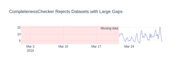
What: Raises InsufficientlyCompleteError if too many values are missing.

Why: Training on heavily incomplete data produces unreliable models.

from openstef_core.exceptions import (
    FlatlinerDetectedError,
    InsufficientlyCompleteError,
    MissingColumnsError,
)
from openstef_models.transforms.validation import CompletenessChecker

checker = CompletenessChecker(columns=["load", "temperature_2m"], completeness_threshold=0.8)

# Good data passes
checker.transform(sample)
print("✓ Complete data passes (threshold=0.8)")

# Incomplete data fails
sparse = sample.data.copy()
sparse.iloc[:2000, sparse.columns.get_loc("temperature_2m")] = np.nan
sparse_ds = TimeSeriesDataset(data=sparse, sample_interval=sample.sample_interval)

try:
    checker.transform(sparse_ds)
except InsufficientlyCompleteError as e:
    print(f"✗ Rejected: {type(e).__name__}")

✓ Complete data passes (threshold=0.8)
✗ Rejected: InsufficientlyCompleteError

Show code cell source

Hide code cell source

# Visualize the incomplete data
fig = go.Figure()
fig.add_trace(
    go.Scatter(
        x=sparse_ds.data.index,
        y=sparse_ds.data["temperature_2m"],
        mode="lines",
        name="Temperature (70% missing at start)",
        line={"width": 1},
    )
)
fig.add_vrect(
    x0=sparse_ds.data.index[0],
    x1=sparse_ds.data.index[2000],
    fillcolor="red",
    opacity=0.1,
    line_width=0,
    annotation_text="Missing data",
)
fig.update_layout(title="CompletenessChecker Rejects Datasets with Large Gaps", height=250, template="plotly_white")
fig.show()

FlatlineChecker

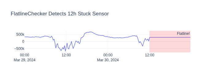
What: Detects constant-value periods (stuck sensors) and raises FlatlinerDetectedError.

Why: A meter stuck at one value for hours is broken. Training on flatlines teaches the model that constant load is normal → bad forecasts.

from openstef_models.transforms.validation import FlatlineChecker

flatliner = FlatlineChecker(
    load_column="load",
    flatliner_threshold=timedelta(hours=6),
    detect_non_zero_flatliner=True,
)

# Normal data passes
flatliner.transform(sample)
print("✓ Normal data passes")

# Inject a 12-hour flatline at end
flat_data = sample.data.copy()
flat_data.iloc[-48:, flat_data.columns.get_loc("load")] = 300000.0
flat_ds = TimeSeriesDataset(data=flat_data, sample_interval=sample.sample_interval)

try:
    flatliner.transform(flat_ds)
except FlatlinerDetectedError as e:
    print(f"✗ Caught: {type(e).__name__}")

✓ Normal data passes
✗ Caught: FlatlinerDetectedError

Show code cell source

Hide code cell source

fig = go.Figure()
fig.add_trace(
    go.Scatter(
        x=flat_ds.data.index[-192:], y=flat_ds.data["load"].iloc[-192:], mode="lines", name="Load", line={"width": 1.5}
    )
)
fig.add_vrect(
    x0=flat_ds.data.index[-48],
    x1=flat_ds.data.index[-1],
    fillcolor="red",
    opacity=0.15,
    line_width=0,
    annotation_text="Flatline!",
)
fig.update_layout(title="FlatlineChecker Detects 12h Stuck Sensor", height=250, template="plotly_white")
fig.show()

InputConsistencyChecker

What: Learns expected columns during fit(), raises error on schema drift.

Why: If a weather source stops providing a column between training and prediction, this catches it before the model produces garbage.

from openstef_models.transforms.validation import InputConsistencyChecker

consistency = InputConsistencyChecker()
consistency.fit(sample)

consistency.transform(sample)
print("✓ Consistent input passes")

# Missing column → caught
reduced = sample.data.drop(columns=["wind_speed_10m"])
reduced_ds = TimeSeriesDataset(data=reduced, sample_interval=sample.sample_interval)
try:
    consistency.transform(reduced_ds)
except MissingColumnsError as e:
    print(f"✗ Caught: {type(e).__name__} - columns changed")

✓ Consistent input passes
✗ Caught: MissingColumnsError - columns changed

---

6. Postprocessing Transforms

These operate on ForecastDataset (after prediction), not training data. They refine model outputs:

Transform	What it does	API Reference
ConfidenceIntervalApplicator	Adds prediction intervals from quantile residuals	ConfidenceIntervalApplicator
IsotonicQuantileCalibrator	Calibrates quantiles via isotonic regression	IsotonicQuantileCalibrator
QuantileSorter	Ensures q10 ≤ q50 ≤ q90	QuantileSorter

See Quantile Calibration for a full walkthrough. Conceptual usage:

from openstef_core.mixins import TransformPipeline
from openstef_models.transforms.postprocessing import (
    ConfidenceIntervalApplicator, QuantileSorter,
)

postprocess = TransformPipeline(transforms=[
    ConfidenceIntervalApplicator(quantiles=[0.1, 0.5, 0.9]),
    QuantileSorter(),
])
calibrated = postprocess.fit_transform(forecast_dataset)

---

7. Building Your Own Transform

All transforms implement TimeSeriesTransform:

• fit(data) — learn parameters (optional for stateless transforms)

• transform(data) — apply transformation

• is_fitted — whether fit() was called

Compose into a TransformPipeline for use in any OpenSTEF workflow.

from typing import override

from pydantic import Field

from openstef_core.base_model import BaseConfig
from openstef_core.transforms import TimeSeriesTransform


class RateOfChangeAdder(BaseConfig, TimeSeriesTransform):
    """Adds rate-of-change (first derivative) as a new column."""

    feature: str = Field(default="load")
    window: int = Field(default=4, description="Periods for differencing.")

    @property
    @override
    def is_fitted(self) -> bool:
        return True  # Stateless

    @override
    def features_added(self) -> list[str]:
        return [f"{self.feature}_roc"]

    @override
    def fit(self, data: TimeSeriesDataset) -> None:
        pass  # Stateless transform — no parameters to learn

    @override
    def transform(self, data: TimeSeriesDataset) -> TimeSeriesDataset:
        df = data.data.copy()
        df[f"{self.feature}_roc"] = df[self.feature].diff(self.window)
        return TimeSeriesDataset(data=df, sample_interval=data.sample_interval)


roc = RateOfChangeAdder(feature="load", window=4)
result = roc.transform(sample)
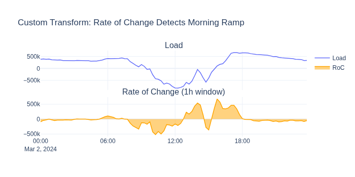
print(f"Large ramps (|roc| > 200kW): {(result.data['load_roc'].abs() > 200000).sum()} timestamps")

Large ramps (|roc| > 200kW): 547 timestamps

Show code cell source

Hide code cell source

one_day = result.data.iloc[96:192]
fig = make_subplots(
    rows=2, cols=1, shared_xaxes=True, vertical_spacing=0.08, subplot_titles=("Load", "Rate of Change (1h window)")
)
fig.add_trace(
    go.Scatter(x=one_day.index, y=one_day["load"], mode="lines", name="Load", line={"width": 1.5}), row=1, col=1
)
fig.add_trace(
    go.Scatter(
        x=one_day.index,
        y=one_day["load_roc"],
        mode="lines",
        name="RoC",
        line={"width": 1.5, "color": "orange"},
        fill="tozeroy",
    ),
    row=2,
    col=1,
)
fig.update_layout(height=350, template="plotly_white", title="Custom Transform: Rate of Change Detects Morning Ramp")
fig.show()

---

8. Composing a Full Pipeline

Order matters: validation → features → cleaning for preprocessing. Postprocessing operates on forecasts and refines model outputs.

Preprocessing pipeline

from openstef_core.mixins import TransformPipeline

preprocessing = TransformPipeline(
    transforms=[
        # 1. Validation
        CompletenessChecker(completeness_threshold=0.5),
        # 2. Feature engineering
        CyclicFeaturesAdder(),
        HolidayFeatureAdder(country_code="NL"),
        DatetimeFeaturesAdder(),
        DaylightFeatureAdder(coordinate=(52.0, 5.9)),
        LagsAdder(
            history_available=timedelta(days=14),
            horizons=horizons,
            add_trivial_lags=False,
            target_column="load",
            custom_lags=[timedelta(days=7)],
            lag_fallback_offset=timedelta(days=7),
        ),
        WindPowerFeatureAdder(windspeed_reference_column="wind_speed_10m"),
        RateOfChangeAdder(feature="load"),
        # 3. Data cleaning
        Imputer(selection=Exclude("load"), imputation_strategy="mean"),
        Scaler(selection=Exclude("load"), method="standard"),
    ]
)

result = preprocessing.fit_transform(sample)
print(
    f"Input: {sample.data.shape[1]} cols → Output: {result.data.shape[1]} cols (+{result.data.shape[1] - sample.data.shape[1]} features)"
)

Input: 28 cols → Output: 58 cols (+30 features)

Postprocessing pipeline

After prediction, postprocessing transforms refine model outputs (e.g., prediction intervals, quantile sorting). These operate on ForecastDataset.

Show code cell source

Hide code cell source

import numpy as np

from openstef_core.datasets import ForecastDataset
from openstef_core.types import Quantile
from openstef_models.transforms.postprocessing import (
    ConfidenceIntervalApplicator,
    QuantileSorter,
)

# Create a synthetic forecast: median prediction = load + small noise
rng = np.random.default_rng(42)
forecast_index = sample.data.index[-192:]  # last 2 days
actuals = sample.data["load"].iloc[-192:]
median_pred = actuals + rng.normal(0, 0.05, len(forecast_index))

# Build a ForecastDataset with median predictions and actuals
forecast_df = pd.DataFrame(
    {"quantile_P50": median_pred, "load": actuals},
    index=forecast_index,
)
forecast_dataset = ForecastDataset(data=forecast_df, sample_interval=sample.sample_interval)

# Fit CI applicator on "validation" data, then add quantile bands
quantiles = [Quantile(0.1), Quantile(0.5), Quantile(0.9)]
postprocessing = TransformPipeline(
    transforms=[
        ConfidenceIntervalApplicator(quantiles=quantiles),
        QuantileSorter(),
    ]
)
calibrated = postprocessing.fit_transform(forecast_dataset)
print(f"Forecast columns: {list(calibrated.data.columns)}")
print(calibrated.data[["quantile_P10", "quantile_P50", "quantile_P90"]].head())

Forecast columns: ['quantile_P50', 'load', 'stdev', 'quantile_P10', 'quantile_P90']
                            quantile_P10   quantile_P50   quantile_P90
timestamp                                                             
2024-03-29 00:00:00+00:00  339999.956363  340000.015236  340000.074108
2024-03-29 00:15:00+00:00  333333.222462  333333.281334  333333.340207
2024-03-29 00:30:00+00:00  333333.311983  333333.370856  333333.429728
2024-03-29 00:45:00+00:00  339999.988156  340000.047028  340000.105901
2024-03-29 01:00:00+00:00  326666.502575  326666.569115  326666.635655

Summary

Group	Transform	Energy forecasting benefit	API
Time	CyclicFeaturesAdder	Smooth daily/weekly encoding	CyclicFeaturesAdder
Time	HolidayFeatureAdder	Avoids overprediction on holidays	HolidayFeatureAdder
Time	LagsAdder	“Last Monday” predicts “this Monday”	LagsAdder
Time	RollingAggregatesAdder	Captures baseline trends	RollingAggregatesAdder
Time	DatetimeFeaturesAdder	Sharp tree splits on peak hours	DatetimeFeaturesAdder
Time	VersionedLagsAdder	Respects data availability for weather lags	VersionedLagsAdder
Weather	DaylightFeatureAdder	Seasonal lighting & solar trends	DaylightFeatureAdder
Weather	AtmosphereDerivedFeaturesAdder	Humidity/density signals	AtmosphereDerivedFeaturesAdder
Weather	RadiationDerivedFeaturesAdder	Tilted irradiance = PV input	RadiationDerivedFeaturesAdder
Energy	WindPowerFeatureAdder	Non-linear power curve	WindPowerFeatureAdder
General	Imputer	Handles missing data	Imputer
General	Scaler	Normalizes feature scales	Scaler
General	OutlierHandler	Enforces plausible ranges	OutlierHandler
General	SampleWeighter	Emphasizes peak loads	SampleWeighter
Validation	CompletenessChecker	Rejects incomplete data	CompletenessChecker
Validation	FlatlineChecker	Catches stuck sensors	FlatlineChecker
Validation	InputConsistencyChecker	Guards schema drift	InputConsistencyChecker
Postprocessing	QuantileSorter	Valid prediction intervals	QuantileSorter

See also

• TransformPipeline — composing transforms

• TimeSeriesTransform — base class

• Building a Custom Pipeline — transforms in a full forecasting model

• Quantile Calibration — postprocessing deep-dive