Foundation Model Forecasting Quickstart

This quickstart produces a zero-shot probabilistic load forecast with the pretrained Chronos-2 model, using OpenSTEF’s ONNX inference backend. There is no training step, and the forecast is conditioned on known weather covariates.

What you’ll do:

• Select a published Chronos-2 checkpoint from the HuggingFace Hub

• Build a forecasting workflow from a config with create_forecasting_workflow

• Feed load history plus known-future weather and read the predicted quantiles

• Plot a P30 / P50 / P70 forecast

• Forecast several origins at once with a single predict_batch call

For what a foundation model is and when to reach for one, see the Foundation Models concept page. For checkpoints, hardware, and backtesting, see the Foundation Model Forecasting guide.

Note

Chronos-2 is zero-shot: it is pretrained and needs no fit(). You give it a window of recent load (and optional known-future weather) and it returns a probabilistic forecast directly. The weather columns cover the whole time range, so the model reads each one as both history and known-future values and can react to, say, an incoming cold day.

Assemble the workflow

ForecastingWorkflowConfig declares the model family, the checkpoint that backs it, the quantiles/horizons to predict, and which columns are the target and the weather covariates. OpenSTEF publishes Chronos-2 as ONNX checkpoints on the HuggingFace Hub; the Chronos2 catalog turns a size into a checkpoint reference, downloaded and cached on first use. The config defaults to the full Chronos2.BASE, so the checkpoint is optional, so here we pick the compact Chronos2.SMALL to keep the tutorial fast and runs in the docs build (pass a LocalCheckpoint(path=...) to run a file on disk). create_forecasting_workflow then resolves the checkpoint, builds the ONNX Runtime session once, and wraps a Chronos2Forecaster in a CustomForecastingWorkflow (a Selector that picks the target and covariates, the forecaster, and a QuantileSorter).

from openstef_core.types import LeadTime, Q
from openstef_foundation_models.models import Chronos2
from openstef_foundation_models.presets.forecasting_workflow import (
    ForecastingWorkflowConfig,
    create_forecasting_workflow,
)
from openstef_models.utils.feature_selection import Include

HORIZON = LeadTime.from_string("P7D")

workflow = create_forecasting_workflow(
    ForecastingWorkflowConfig(
        model="chronos2",
        checkpoint=Chronos2.SMALL.checkpoint(),
        quantiles=[Q(0.3), Q(0.5), Q(0.7)],
        horizons=[HORIZON],
        target_column="load",
        # Keep the target plus the three known-future weather covariates; every
        # kept non-target column is forwarded to Chronos-2 as a covariate.
        selected_features=Include(
            "load",
            "shortwave_radiation",
            "wind_speed_80m",
            "temperature_2m",
        ),
    )
)

# Zero-shot: the model is "fitted" on construction - there is nothing to train.
print(f"is_fitted: {workflow.model.is_fitted}")
print(f"quantiles: {workflow.model.quantiles}")

2026-07-10 06:54:05.864216114 [W:onnxruntime:Default, device_discovery.cc:133 GetPciBusId] Skipping pci_bus_id for PCI path at "/sys/devices/LNXSYSTM:00/LNXSYBUS:00/ACPI0004:00/MSFT1000:00/5620e0c7-8062-4dce-aeb7-520c7ef76171" because filename "5620e0c7-8062-4dce-aeb7-520c7ef76171" did not match expected pattern of [0-9a-f]+:[0-9a-f]+:[0-9a-f]+[.][0-9a-f]+

Warning: You are sending unauthenticated requests to the HF Hub. Please set a HF_TOKEN to enable higher rate limits and faster downloads.

[2026-07-10 06:54:07,226][INFO] DefaultProviderPolicy selected execution-provider chain ['CPUExecutionProvider'] for checkpoint 'chronos2' (precision=fp32, static_shapes=False) on linux.

[2026-07-10 06:54:07,559][INFO] ONNX Runtime session built; realized providers: ['CPUExecutionProvider'].

is_fitted: True
quantiles: [0.3, 0.5, 0.7]

Load real load history and weather

We reuse the Liander 2024 benchmark dataset for a realistic medium-voltage feeder load series together with its weather forecasts. The workflow’s Selector keeps the target (load) and the three weather covariates; everything else is ignored.

We take 60 days of history up to a chosen forecast start and keep the weather columns running through the 7-day horizon, so Chronos-2 can use the known-future weather as a covariate.

from datetime import datetime, timedelta

from openstef_core.testing import load_liander_dataset

dataset = load_liander_dataset()

forecast_start = datetime.fromisoformat("2024-11-15T00:00:00Z")
context_start = forecast_start - timedelta(days=60)

# The window spans history + horizon: load history conditions the model, while the
# weather columns are known across the whole range (history and future).
window = dataset.filter_by_range(start=context_start, end=forecast_start + HORIZON.value)

print(f"Window:   {context_start:%Y-%m-%d} to {forecast_start + HORIZON.value:%Y-%m-%d}, {len(window.data):,} rows")

Window:   2024-09-16 to 2024-11-22, 6,432 rows

Forecast

workflow.predict selects the target and covariates, runs the ONNX session once, and post-processes the output: it slices the model’s frozen horizon to the requested 7 days and resamples Chronos-2’s native quantile grid onto the requested P30 / P50 / P70.

forecast = workflow.predict(window, forecast_start=forecast_start)

print(f"Forecast rows: {len(forecast.data)}")
print(f"Quantiles:     {forecast.quantiles}")
forecast.data.head()

Forecast rows: 672
Quantiles:     [0.3, 0.5, 0.7]

	quantile_P30	quantile_P50	quantile_P70	load
timestamp
2024-11-15 00:00:00+00:00	333879.03125	342650.71875	351709.84375	336666.666667
2024-11-15 00:15:00+00:00	328176.90625	336179.78125	343998.84375	340000.000000
2024-11-15 00:30:00+00:00	321083.00000	331317.34375	339581.93750	320000.000000
2024-11-15 00:45:00+00:00	318212.25000	328051.59375	337488.40625	320000.000000
2024-11-15 01:00:00+00:00	312202.90625	322877.06250	332967.43750	313333.333333

Visualize the forecast

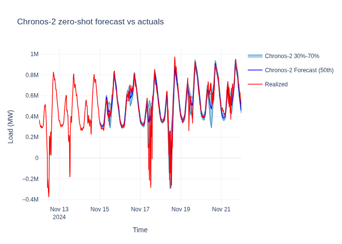
ForecastTimeSeriesPlotter overlays the actual load against the median forecast with a shaded quantile band.

Show code cell source

Hide code cell source

from openstef_beam.analysis.plots import ForecastTimeSeriesPlotter

actuals = dataset.filter_by_range(
    start=forecast_start - timedelta(days=3),
    end=forecast_start + HORIZON.value,
).data["load"]

fig = (
    ForecastTimeSeriesPlotter()
    .add_measurements(measurements=actuals)
    .add_model(
        model_name="Chronos-2",
        forecast=forecast.median_series,
        quantiles=forecast.quantiles_data,
    )
    .plot()
)
fig = cast(Any, fig)
fig.update_layout(
    title="Chronos-2 zero-shot forecast vs actuals",
    yaxis_title="Load (MW)",
    xaxis_title="Time",
    height=500,
)
fig.show()

Forecast many origins in one call

A foundation model handles many series or origins in one pass. Instead of looping predict per window, hand the whole batch to predict_batch: it concatenates the windows and runs the ONNX session once, returning one forecast per window in input order. The numbers match the serial loop; only throughput changes.

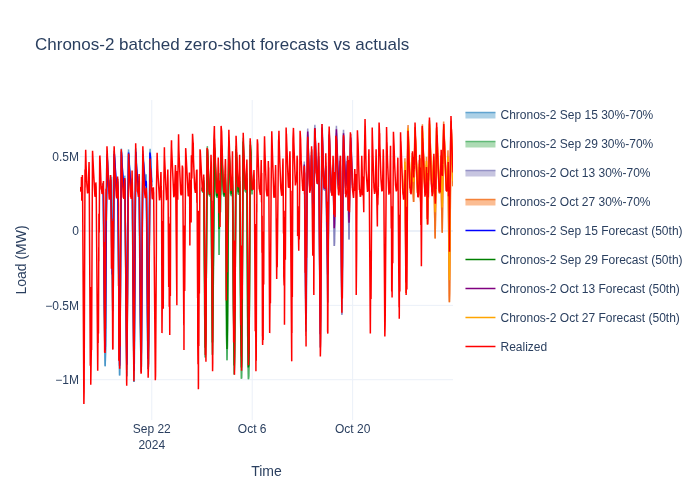
Here we carve four forecast origins two weeks apart out of the same dataset. This is handy for backtesting; in a live setting you would more often forecast many different locations or targets at once. Each window keeps its own 60 days of history plus the 7-day horizon of known-future weather.

forecast_starts = [
    datetime.fromisoformat("2024-09-15T00:00:00Z"),
    datetime.fromisoformat("2024-09-29T00:00:00Z"),
    datetime.fromisoformat("2024-10-13T00:00:00Z"),
    datetime.fromisoformat("2024-10-27T00:00:00Z"),
]
windows = [
    dataset.filter_by_range(start=start - timedelta(days=60), end=start + HORIZON.value) for start in forecast_starts
]

batched = workflow.predict_batch(windows, forecast_start=forecast_starts)
print(f"Forecasts returned: {len(batched)} (one backend call for the whole batch)")

Forecasts returned: 4 (one backend call for the whole batch)

Each window is an independent 7-day forecast. We overlay the four median forecasts against the actual load to see how the same zero-shot model tracks the series at different points in time.

Show code cell source

Hide code cell source

batch_actuals = dataset.filter_by_range(
    start=forecast_starts[0] - timedelta(days=3),
    end=forecast_starts[-1] + HORIZON.value,
).data["load"]

batch_plotter = ForecastTimeSeriesPlotter().add_measurements(measurements=batch_actuals)
for start, batch_forecast in zip(forecast_starts, batched, strict=True):
    batch_plotter = batch_plotter.add_model(
        model_name=f"Chronos-2 {start:%b %d}",
        forecast=batch_forecast.median_series,
        quantiles=batch_forecast.quantiles_data,
    )

fig = cast(Any, batch_plotter.plot())
fig.update_layout(
    title="Chronos-2 batched zero-shot forecasts vs actuals",
    yaxis_title="Load (MW)",
    xaxis_title="Time",
    height=500,
)
fig.show()

Next steps

• Foundation Model Forecasting guide: pick a checkpoint, run one from disk, choose the execution provider for your hardware, and backtest with openstef-beam.

• Forecasting Quickstart: train a gradient-boosted model and compare it against this zero-shot baseline.

• Foundation Models concept page: what a foundation model is and when to prefer it over a trained model.