Understanding Time Series Datasets

Imagine it is 08:00 UTC on December 27, 2024. You need to forecast electricity load for a medium-voltage substation in Gorredijk (NL) over the next 48 hours. What data can you use?

The answer depends on when data became available - not just what timestamps it describes. A weather forecast issued at 06:00 today describes tomorrow’s temperature, but a forecast issued tomorrow morning describes the same moment more accurately. Using future-issued data during training causes data leakage.

OpenSTEF prevents this with TimeSeriesDataset - a thin wrapper around a pandas.DataFrame that adds a timestamp index and an available_at column recording when each row became known. By filtering on available_at, you guarantee that only genuinely available data enters the model.

This notebook walks through a real forecasting scenario using the Liander distribution network dataset, building from a single data source up to a multi-source forecasting pipeline.

Show code cell source

Hide code cell source

import logging
import warnings
from datetime import UTC, datetime, timedelta
from pathlib import Path

import pandas as pd
import plotly.graph_objects as go
from plotly.subplots import make_subplots

from openstef_core.testing import configure_notebook_display, load_liander_dataset, setup_notebook_logging

configure_notebook_display()
setup_notebook_logging()

# Suppress noisy HTTP and progress-bar warnings
logging.getLogger("httpx").setLevel(logging.WARNING)
logging.getLogger("httpcore").setLevel(logging.WARNING)
warnings.filterwarnings("ignore", category=FutureWarning)
warnings.filterwarnings("ignore", message="IProgress not found")

# Download dataset
data_dir = Path("liander_dataset")
load_liander_dataset(local_dir=data_dir)

from openstef_core.datasets import TimeSeriesDataset, VersionedTimeSeriesDataset
from openstef_core.types import AvailableAt, LeadTime

load = TimeSeriesDataset.read_parquet(data_dir / "load_measurements" / "mv_feeder" / "OS Gorredijk.parquet")
epex = TimeSeriesDataset.read_parquet(data_dir / "EPEX.parquet")
profiles = TimeSeriesDataset.read_parquet(data_dir / "profiles.parquet")
weather = TimeSeriesDataset.read_parquet(
    data_dir / "weather_forecasts_versioned" / "mv_feeder" / "OS Gorredijk.parquet"
)

How versioning works

Every row in a TimeSeriesDataset has two time references:

• index (timestamp) - the moment this row describes

• available_at - the moment this row became known

The gap between them is the lead time. Let’s look at one timestamp:

sample_ts = pd.Timestamp("2024-12-28 12:00", tz="UTC")
weather.data.loc[[sample_ts], ["temperature_2m", "available_at"]]

	temperature_2m	available_at
timestamp
2024-12-28 12:00:00+00:00	0.2805	2024-12-28 12:00:00+00:00
2024-12-28 12:00:00+00:00	1.1805	2024-12-27 12:00:00+00:00
2024-12-28 12:00:00+00:00	3.6500	2024-12-26 12:00:00+00:00
2024-12-28 12:00:00+00:00	4.1000	2024-12-25 12:00:00+00:00
2024-12-28 12:00:00+00:00	7.0000	2024-12-24 12:00:00+00:00
2024-12-28 12:00:00+00:00	5.1500	2024-12-23 12:00:00+00:00

Six forecast runs predicted the same moment. The earliest was issued five days ahead (long lead time), the latest was same-day (short lead time). Each version refines the prediction as the event approaches.

The forecasting challenge: December 28

December 28, 2024 brought below-normal temperatures to northern Netherlands. How did the six forecast versions perform?

Show code cell source

Hide code cell source

weather_raw = pd.read_parquet(data_dir / "weather_forecasts_versioned" / "mv_feeder" / "OS Gorredijk.parquet")

dec28 = weather_raw[(weather_raw["timestamp"] >= "2024-12-28") & (weather_raw["timestamp"] < "2024-12-29")].copy()
dec28["version_date"] = dec28["available_at"].dt.date

colors_versions = ["#94a3b8", "#64748b", "#f59e0b", "#ea580c", "#dc2626", "#2563eb"]
labels = [
    "5 days before (Dec 23)",
    "4 days before (Dec 24)",
    "3 days before (Dec 25)",
    "2 days before (Dec 26)",
    "1 day before (Dec 27)",
    "Same day (Dec 28)",
]

fig = go.Figure()
for i, (vdate, label, color) in enumerate(
    zip(sorted(dec28["version_date"].unique()), labels, colors_versions, strict=False)
):
    subset = dec28[dec28["version_date"] == vdate].sort_values("timestamp")
    fig.add_trace(
        go.Scatter(
            x=subset["timestamp"],
            y=subset["temperature_2m"],
            mode="lines",
            name=label,
            line={"color": color, "width": 2 if i < 5 else 3},
            opacity=0.6 if i < 4 else 1.0,
        )
    )

fig.update_layout(
    title="Temperature forecasts for December 28 - six versions compared",
    xaxis_title="Time (UTC)",
    yaxis_title="Temperature (C)",
    height=420,
    margin={"t": 50, "b": 40},
    legend={"x": 0.01, "y": 0.99, "bgcolor": "rgba(255,255,255,0.8)"},
)
fig.show()

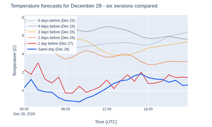
The spread between versions is significant: early forecasts predicted warmer conditions than later ones. Let’s quantify that spread:

Show code cell source

Hide code cell source

spread = dec28.groupby("timestamp")["temperature_2m"].agg(["min", "max", "mean"])
spread["range"] = spread["max"] - spread["min"]

fig = make_subplots(
    rows=2,
    cols=1,
    shared_xaxes=True,
    vertical_spacing=0.08,
    subplot_titles=("Temperature: all versions vs mean", "Spread across versions"),
)

fig.add_trace(
    go.Scatter(
        x=spread.index,
        y=spread["max"],
        mode="lines",
        line={"width": 0},
        showlegend=False,
    ),
    row=1,
    col=1,
)
fig.add_trace(
    go.Scatter(
        x=spread.index,
        y=spread["min"],
        mode="lines",
        line={"width": 0},
        fill="tonexty",
        fillcolor="rgba(37, 99, 235, 0.2)",
        name="Version range",
    ),
    row=1,
    col=1,
)
fig.add_trace(
    go.Scatter(
        x=spread.index,
        y=spread["mean"],
        mode="lines",
        line={"color": "#2563eb", "width": 2},
        name="Mean across versions",
    ),
    row=1,
    col=1,
)

fig.add_trace(
    go.Bar(
        x=spread.index,
        y=spread["range"],
        marker_color="#ea580c",
        opacity=0.7,
        name="Spread (C)",
    ),
    row=2,
    col=1,
)

fig.update_layout(height=450, margin={"t": 50, "b": 40})
fig.update_yaxes(title_text="C", row=1, col=1)
fig.update_yaxes(title_text="C", row=2, col=1)
fig.show()

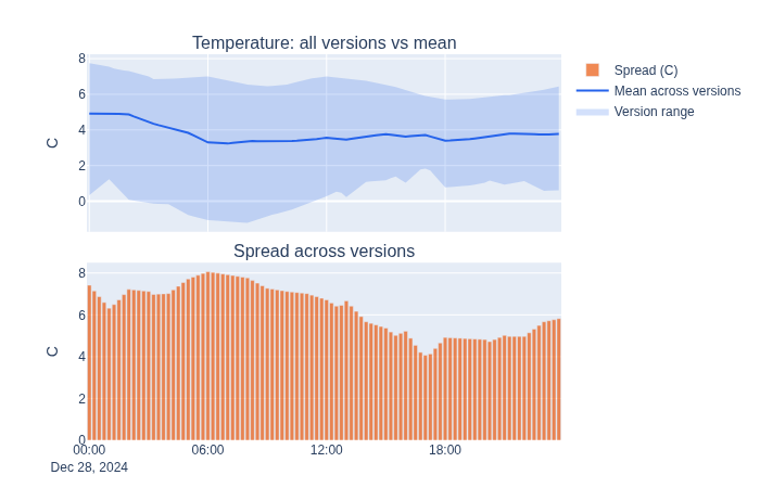
The spread exceeds 2 degrees C during parts of the day - a direct measure of forecast uncertainty. Large divergence means the weather model was still converging on the actual outcome.

At our decision point (Dec 27, 08:00), we can only use the “1 day before” version. The “same day” version does not exist yet. Without tracking available_at, we might accidentally use it during training.

Filtering: what was genuinely available?

TimeSeriesDataset provides three filter methods to enforce data availability constraints:

Method	Question it answers
filter_by_available_before()	What existed at a specific moment?
filter_by_available_at()	What matches a recurring operational schedule?
filter_by_lead_time()	What has at least N hours of advance notice?

To demonstrate clearly, let’s build a synthetic dataset where forecasts are issued every 3 hours; each run covers the next 72 hours. This produces a rich distribution of lead times:

Show code cell source

Hide code cell source

import numpy as np

# Generate synthetic forecasts: 8 runs/day, each covering 72h ahead (15-min steps)
rng = np.random.default_rng(42)
issue_times = pd.date_range("2024-12-20", "2024-12-27 21:00", freq="3h", tz="UTC")
target_times = pd.date_range("2024-12-20", "2024-12-29", freq="15min", tz="UTC")

rows = []
for issue in issue_times:
    targets_in_range = target_times[(target_times > issue) & (target_times <= issue + pd.Timedelta(hours=72))]
    rows.extend(
        {"timestamp": t, "available_at": issue, "temperature_2m": rng.normal(3.0, 2.0)} for t in targets_in_range
    )

synth_df = pd.DataFrame(rows).set_index("timestamp")
synth_weather = TimeSeriesDataset(synth_df, sample_interval=timedelta(minutes=15))
print(
    f"Synthetic dataset: {len(synth_weather.data):,} rows, "
    f"{synth_weather.data.index.nunique():,} unique timestamps, "
    f"~{len(synth_weather.data) // synth_weather.data.index.nunique()} versions/timestamp"
)

Synthetic dataset: 16,992 rows, 864 unique timestamps, ~19 versions/timestamp

now = datetime(2024, 12, 27, 8, 0, tzinfo=UTC)

# Point-in-time: only rows that existed by Dec 27 08:00
snapshot_synth = synth_weather.filter_by_available_before(now)

# Operational schedule: only rows available by 06:00 the day before the target
day_ahead_synth = synth_weather.filter_by_available_at(AvailableAt.from_string("D-1T0600"))

# Minimum lead time: at least 24h between issuance and target
long_lead_synth = synth_weather.filter_by_lead_time(LeadTime.from_string("P1D"))

Show code cell source

Hide code cell source

def lead_hours(tsd: TimeSeriesDataset) -> pd.Series:
    """Return positive lead times in hours.

    Returns:
        Series of lead times where the forecast was issued before the target timestamp.
    """
    h = (tsd.data.index - tsd.data["available_at"]).dt.total_seconds() / 3600
    return h[h > 0]


fig = make_subplots(
    rows=1,
    cols=3,
    subplot_titles=(
        f"available_before<br><sup>Dec 27 08:00 | {len(snapshot_synth.data):,} rows</sup>",
        f"available_at<br><sup>'D-1T0600' | {len(day_ahead_synth.data):,} rows</sup>",
        f"lead_time<br><sup>'P1D' | {len(long_lead_synth.data):,} rows</sup>",
    ),
    horizontal_spacing=0.08,
)

datasets_filtered = [snapshot_synth, day_ahead_synth, long_lead_synth]
colors_filt = ["#2563eb", "#059669", "#ea580c"]

for col, tsd, color in zip([1, 2, 3], datasets_filtered, colors_filt, strict=False):
    h = lead_hours(tsd)
    fig.add_trace(
        go.Histogram(
            x=h,
            nbinsx=50,
            marker_color=color,
            opacity=0.8,
            showlegend=False,
        ),
        row=1,
        col=col,
    )

fig.update_xaxes(title_text="Lead time (hours)", range=[0, 96])
fig.update_yaxes(title_text="Row count", col=1)
fig.update_layout(height=320, margin={"t": 70, "b": 50})
fig.show()

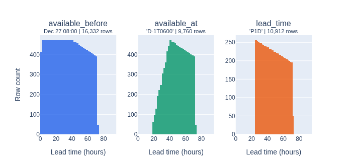
The three filters produce distinctly different lead-time distributions:

• available_before keeps everything issued before our decision point – a uniform spread of lead times from 0 to 72 hours.

• available_at (D-1T0600) enforces a recurring operational window - only forecasts available by yesterday 06:00 survive, shifting the distribution toward longer lead times (>18h).

• lead_time (P1D) removes all rows with less than 24 hours of advance notice, producing a hard cutoff.

Now let’s apply the same filters to our real weather data and resolve versions:

Resolving versions with select_version

After filtering, we still have multiple versions per timestamp. Models need exactly one row per timestamp. select_version() picks the freshest (most recent available_at) row for each timestamp:

now = datetime(2024, 12, 27, 8, 0, tzinfo=UTC)
snapshot = weather.filter_by_available_before(now)

Show code cell source

Hide code cell source

# Show before/after for a few timestamps
sample_range_filtered = snapshot.data.loc["2024-12-28 10:00":"2024-12-28 12:00"]

Before select_version - multiple versions per timestamp:

Show code cell source

Hide code cell source

print(f"  ({len(sample_range_filtered)} rows for 3 hours)")
sample_range_filtered[["temperature_2m", "available_at"]].head(12)

  (36 rows for 3 hours)

	temperature_2m	available_at
timestamp
2024-12-28 10:00:00+00:00	4.2000	2024-12-26 10:00:00+00:00
2024-12-28 10:00:00+00:00	5.0000	2024-12-25 10:00:00+00:00
2024-12-28 10:00:00+00:00	6.5500	2024-12-24 10:00:00+00:00
2024-12-28 10:00:00+00:00	4.9000	2024-12-23 10:00:00+00:00
2024-12-28 10:15:00+00:00	4.1125	2024-12-26 10:15:00+00:00
2024-12-28 10:15:00+00:00	4.8750	2024-12-25 10:15:00+00:00
2024-12-28 10:15:00+00:00	6.6250	2024-12-24 10:15:00+00:00
2024-12-28 10:15:00+00:00	4.9375	2024-12-23 10:15:00+00:00
2024-12-28 10:30:00+00:00	4.0250	2024-12-26 10:30:00+00:00
2024-12-28 10:30:00+00:00	4.7500	2024-12-25 10:30:00+00:00
2024-12-28 10:30:00+00:00	6.7000	2024-12-24 10:30:00+00:00
2024-12-28 10:30:00+00:00	4.9750	2024-12-23 10:30:00+00:00

After select_version - one row per timestamp, no available_at column:

resolved = snapshot.select_version()
print(f"  {len(snapshot.data):,} rows -> {len(resolved.data):,} rows")
resolved.data.loc["2024-12-28 10:00":"2024-12-28 12:00", ["temperature_2m"]].head(9)

  199,734 rows -> 35,169 rows

	temperature_2m
timestamp
2024-12-28 10:00:00+00:00	4.2000
2024-12-28 10:15:00+00:00	4.1125
2024-12-28 10:30:00+00:00	4.0250
2024-12-28 10:45:00+00:00	3.9375
2024-12-28 11:00:00+00:00	3.8500
2024-12-28 11:15:00+00:00	3.8000
2024-12-28 11:30:00+00:00	3.7500
2024-12-28 11:45:00+00:00	3.7000
2024-12-28 12:00:00+00:00	3.6500

Notice two things:

1. For each timestamp, select_version kept the row with the latest available_at - the most up-to-date information that passed the filter.

2. The available_at column is gone. The result is a plain DataFrame indexed by timestamp - ready for feature engineering and model training.

This resolution is intentionally lossy: you commit to one version per timestamp and discard the rest.

Non-versioned datasets

Not all sources have multiple versions. EPEX prices and load measurements have exactly one row per timestamp - they are non-versioned:

print(f"EPEX versioned: {epex.is_versioned}  (rows: {len(epex.data):,})")
print(f"Load versioned: {load.is_versioned}  (rows: {len(load.data):,})")

# select_version is safe to call on any TimeSeriesDataset - it's a no-op here
flat_epex = epex.select_version()
print(f"\nEPEX after select_version: {len(flat_epex.data):,} rows (unchanged)")

EPEX versioned: True  (rows: 35,136)
Load versioned: True  (rows: 35,136)

EPEX after select_version: 35,136 rows (unchanged)

You can also create a non-versioned TimeSeriesDataset from any DataFrame with a DatetimeIndex:

# Build a simple non-versioned dataset from scratch
measurements = pd.DataFrame(
    {"power_kw": [100, 120, 115, 108, 95]},
    index=pd.date_range("2025-01-01", periods=5, freq="15min", tz="UTC"),
)
tsd_simple = TimeSeriesDataset(measurements, sample_interval=timedelta(minutes=15))
print(f"Features:  {tsd_simple.feature_names}")
print(f"Versioned: {tsd_simple.is_versioned}")

Features:  ['power_kw']
Versioned: False

# Build a versioned dataset by adding an available_at column
forecasts = pd.DataFrame(
    {
        "temperature": [2.1, 1.8, 1.5, 1.2],
        "available_at": pd.to_datetime(
            [
                "2025-01-01 00:00",
                "2025-01-01 06:00",  # two versions for 12:00
                "2025-01-01 00:00",
                "2025-01-01 06:00",  # two versions for 12:15
            ],
            utc=True,
        ),
    },
    index=pd.DatetimeIndex(
        ["2025-01-01 12:00", "2025-01-01 12:00", "2025-01-01 12:15", "2025-01-01 12:15"],
        tz="UTC",
    ),
)
tsd_versioned = TimeSeriesDataset(forecasts, sample_interval=timedelta(minutes=15))
print(f"Features:  {tsd_versioned.feature_names}")
print(f"Versioned: {tsd_versioned.is_versioned}")

Features:  ['temperature']
Versioned: True

The data sources

So far we have focused on weather, but a load forecast also needs energy prices, standard profiles, and historical load measurements. The Liander dataset contains four sources, each stored as a TimeSeriesDataset:

summary = pd.DataFrame({
    "Source": ["Load", "Weather", "EPEX prices", "Profiles"],
    "Features": [
        ", ".join(load.feature_names),
        f"{len(weather.feature_names)} variables",
        ", ".join(epex.feature_names),
        f"{len(profiles.feature_names)} profiles",
    ],
    "Rows": [len(load.data), len(weather.data), len(epex.data), len(profiles.data)],
    "Versioned": [load.is_versioned, weather.is_versioned, epex.is_versioned, profiles.is_versioned],
    "Update schedule": ["real-time", "every ~6h", "noon day-before", "months ahead"],
})
summary.set_index("Source").style.set_properties(padding="6px 12px")

	Features	Rows	Versioned	Update schedule
Source
Load	load	35136	True	real-time
Weather	11 variables	201534	True	every ~6h
EPEX prices	EPEX_NL	35136	True	noon day-before
Profiles	15 profiles	35136	True	months ahead

These sources update on different schedules - weather has ~6 versions per timestamp, EPEX has one, and profiles never change. A naive DataFrame join would create a cross-product explosion.

Combining sources: VersionedTimeSeriesDataset

VersionedTimeSeriesDataset solves this by keeping each source as a separate part and only joining them when you explicitly resolve. This is especially important for backtesting, where the system replays historical decisions: at each past decision point, the filters reconstruct exactly what was available, so backtested performance reflects real operational conditions.

Let’s combine weather and EPEX prices:

combined = VersionedTimeSeriesDataset([weather, epex])
print(f"Parts:     {len(combined.data_parts)}")
print(f"Timestamps: {len(combined.index):,}")
print(f"Features:  {combined.feature_names[:3]} ... {combined.feature_names[-1]}")

Parts:     2
Timestamps: 35,229
Features:  ['temperature_2m', 'relative_humidity_2m', 'surface_pressure'] ... EPEX_NL

The same filter_by_* methods work here - they apply the constraint to each part independently:

filtered_combined = combined.filter_by_available_before(now)
print(f"Weather part: {len(filtered_combined.data_parts[0].data):,} rows")
print(f"EPEX part:    {len(filtered_combined.data_parts[1].data):,} rows")

Weather part: 199,734 rows
EPEX part:    34,748 rows

Resolving to flat data

select_version() resolves each part (picks freshest version) then joins along columns into a single flat TimeSeriesDataset:

flat = filtered_combined.select_version()
print(f"Result: {type(flat).__name__} with {len(flat.data):,} rows")
print(f"Columns: {list(flat.data.columns[:5])} ...")

Result: TimeSeriesDataset with 35,229 rows
Columns: ['temperature_2m', 'relative_humidity_2m', 'surface_pressure', 'cloud_cover', 'wind_speed_10m'] ...

For models that need to train at multiple lead times (e.g. 1h, 4h, 24h ahead), to_horizons() applies lead-time filtering + version selection for each horizon and stacks the results. The output has a horizon column:

horizons = [LeadTime.from_string("PT1H"), LeadTime.from_string("PT4H"), LeadTime.from_string("P1D")]
horizon_data = combined.to_horizons(horizons)
print(f"Shape: {horizon_data.data.shape}")
print(f"Horizons: {horizon_data.data['horizon'].unique().tolist()}")

Shape: (105687, 13)
Horizons: [Timedelta('0 days 01:00:00'), Timedelta('0 days 04:00:00'), Timedelta('1 days 00:00:00')]

Summary

Concept	Role
TimeSeriesDataset	One data source: timestamp index + available_at + features
VersionedTimeSeriesDataset	Multiple sources with different update schedules
filter_by_*	Restrict to genuinely available data (works on both types)
select_version()	Pick freshest version per timestamp (lossy)
to_horizons()	Resolve at fixed lead times for multi-horizon training

The workflow:

1. Load sources as TimeSeriesDataset instances

2. Filter to enforce what was available at prediction time

3. Resolve versions with select_version() for single-source work

4. Combine with VersionedTimeSeriesDataset when multiple sources are needed

5. Resolve to flat data with select_version() or to_horizons()