BEAM#

Energy forecasting teams need to compare models fairly. A model that appears superior on one target or time horizon may underperform on another. Without a systematic framework, comparisons become ad-hoc: different evaluation windows, inconsistent data splits, or accidental future data leakage can all invalidate results. BEAM (Backtesting, Evaluation, Analysis, and Metrics) solves this by providing a reproducible, sequential pipeline for model comparison.

This page explains the architecture and design principles of BEAM. For a hands-on walkthrough, see the Backtesting Quickstart.

Why Systematic Benchmarking Matters#

In production energy forecasting, you must answer questions like:

Does a new model outperform the current one across all targets?
How does performance vary by lead time (1-hour ahead vs. day-ahead)?
Are improvements consistent across seasonal windows?

Answering these requires three guarantees:

No future data leakage during backtesting (the model must never see data it would not have in production).
Consistent segmentation of results by horizon, availability time, and evaluation window.
Reproducible analysis that can be re-run or extended without re-executing expensive training.

BEAM encodes these guarantees into its pipeline structure.

Pipeline Overview#

BEAM is organized as three sequential stages, orchestrated by BenchmarkPipeline:

        graph LR
    TP[TargetProvider] -->|ground truth & predictors| BT[BacktestPipeline]
    FF[ForecasterFactory] --> BT
    BT -->|TimeSeriesDataset| EV[EvaluationPipeline]
    EV -->|EvaluationReport| AN[AnalysisPipeline]
    TP -->|ground truth| EV
    VP[VisualizationProviders] --> AN
    BT --> ST[(BenchmarkStorage)]
    EV --> ST
    AN --> ST
    AN --> AO[AnalysisOutput]
    classDef primary fill:#00D9C5,stroke:#1E3A5F,stroke-width:2px,color:#000
    classDef secondary fill:#1E3A5F,stroke:#00D9C5,stroke-width:2px,color:#fff
    classDef accent fill:#e6f7f5,stroke:#00D9C5,stroke-width:2px,color:#000
    class BT,EV,AN primary
    class TP,FF,VP secondary
    class ST,AO accent

BEAM Pipeline Stages#
Stage	Responsibility	Input	Output
BacktestPipeline	Simulate production forecasting over historical data	Ground truth, predictors, BacktestForecasterMixin	`TimeSeriesDataset` of predictions
EvaluationPipeline	Segment predictions and compute metrics	Predictions, ground truth, metric providers	`EvaluationReport`
AnalysisPipeline	Generate visualizations at configurable aggregation levels	EvaluationReports, VisualizationProviders	`AnalysisOutput`

These stages are completely decoupled. You can re-run evaluation with different metrics without re-running the backtest, or generate new visualizations without recomputing metrics. This decoupling matters because each stage has a different computational cost and a different rate of change:

Backtesting is expensive. Every backtest requires many forward passes through the model, potentially with periodic retraining. You want to run this once and re-use the predictions.
You may not need backtesting at all. If you ran backtests with external tooling, received shared predictions from a colleague, or already have stored results from a previous run, you can feed them directly into evaluation.
Evaluation and analysis evolve independently. As you refine your metric set or add new visualization providers, you should not have to wait hours re-running expensive model predictions.

Backtesting Stage#

The BacktestPipeline simulates how a model would have performed in production by stepping through historical data sequentially. In production, forecasts are generated at regular intervals (e.g., every 6 hours) and models are retrained periodically (e.g., weekly). The simulation replicates this schedule so that error distributions match what you would observe in a real deployment.

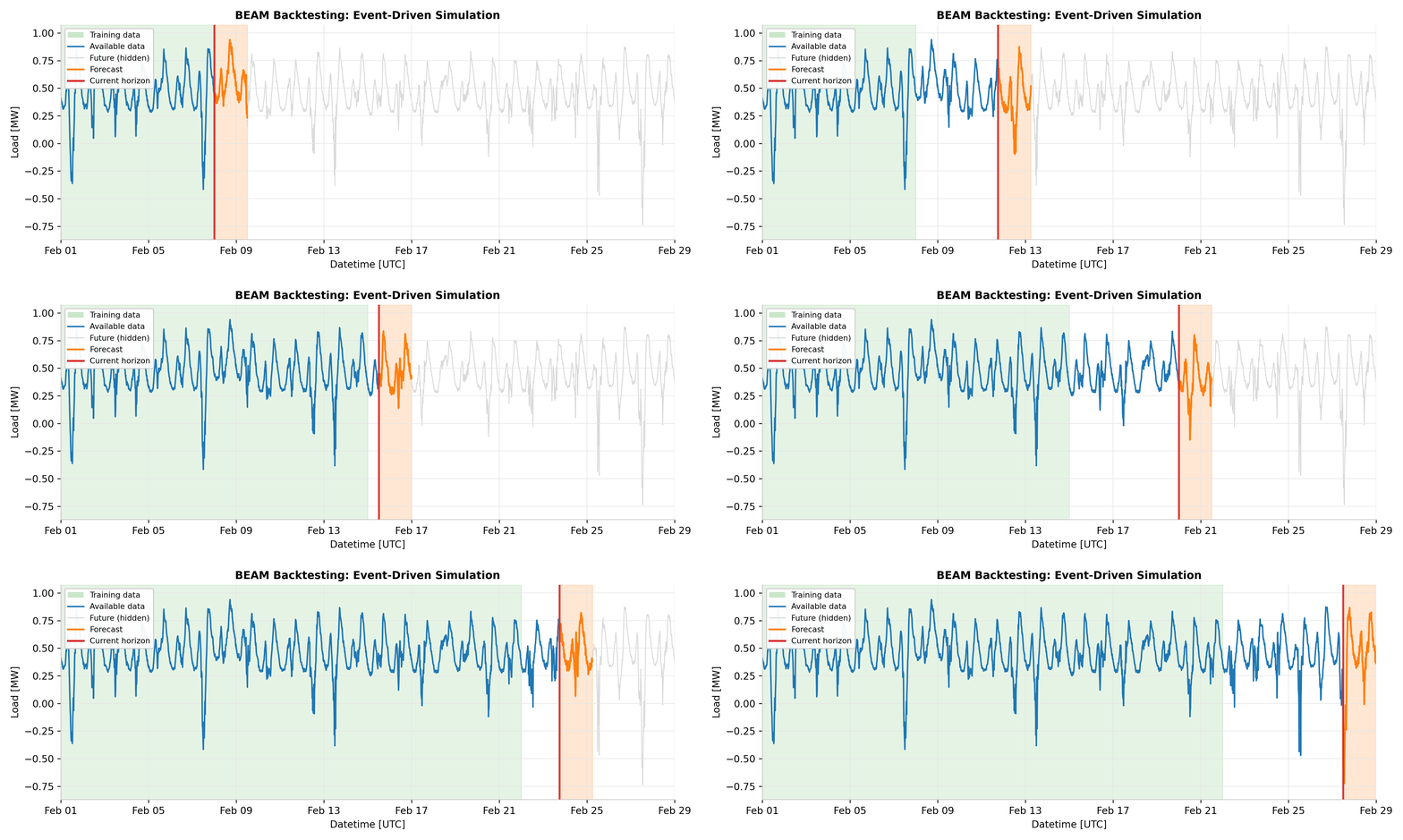
Animation showing BEAM stepping through time - green region marks training data, orange line shows forecast output, red line marks the current horizon.

Preventing future data leakage. The central design challenge in backtesting is ensuring the model never accesses data from the future. Energy data has different arrival latencies: weather forecast revisions, late meter readings, and market settlements all arrive at different times. BEAM uses RestrictedHorizonVersionedTimeSeries to track not just data values but when each value first became available, restricting the model’s view to only data published before the simulated “current time”.

Warning

A BacktestForecasterMixin is not the same as a Forecaster in openstef-models. It is glue code that adapts any model to the backtesting interface, receiving only a restricted data view and never having direct access to the full dataset.

Event-driven simulation. BacktestEventGenerator schedules train and predict events according to the configured predict_interval and train_interval. It merges two streams of events in chronological order, with train events always executing before predict events at the same timestamp (ensuring the model is freshly trained before generating predictions). For each event, the pipeline calls fit() or predict() on the forecaster, always passing a RestrictedHorizonVersionedTimeSeries that enforces the temporal boundary.

The output is a TimeSeriesDataset containing all predictions, each tagged with an available_at timestamp indicating when that prediction would have been generated in production.

Evaluation Stage#

The EvaluationPipeline is entirely separate from backtesting. It takes predictions and ground truth, then segments and scores them along three dimensions. Each dimension answers a different operational question:

available_at: When the prediction was generated (e.g., “day-ahead at 06:00”). A model may perform differently when forecasting in the morning versus the evening because different information is available at each time.
lead_time: The gap between prediction generation and the target timestamp (e.g., 36 hours ahead). Model error typically grows with the forecast horizon, so a “better” model might only outperform at short lead times.
time_windows: Rolling evaluation periods (e.g., 21-day windows). Seasonal effects and model drift mean that aggregate metrics can hide periods of poor performance.

Configurable metrics. Metrics are supplied as provider objects. BEAM includes providers such as RMAEProvider (Relative Mean Absolute Error) and RCRPSProvider (Relative Continuous Ranked Probability Score) for probabilistic evaluation. You can implement custom providers to add domain-specific metrics.

from openstef_beam.evaluation import EvaluationConfig, EvaluationPipeline
from openstef_beam.evaluation.metric_providers import RMAEProvider, RCRPSProvider

eval_pipeline = EvaluationPipeline(
    config=EvaluationConfig(),
    quantiles=forecaster.quantiles,
    window_metric_providers=[RMAEProvider(), RCRPSProvider()],
    global_metric_providers=[RMAEProvider(), RCRPSProvider()],
)

The output is an EvaluationReport containing per-subset metrics that can be inspected programmatically or passed to the analysis stage.

Analysis Stage#

The AnalysisPipeline transforms evaluation reports into HTML visualizations. It operates at configurable aggregation levels:

Aggregation Levels#
Level	Description
NONE	Single run, single target - individual performance analysis
TARGET	Single run, per target - cross-target comparison (e.g., RMAE per target)
GROUP	Single run, multiple targets - cross-group comparison (e.g., RMAE per group)
RUN_AND_NONE	Multiple runs, single target - compare model variants on one target
RUN_AND_TARGET	Multiple runs, per target - compare model variants across targets
RUN_AND_GROUP	Multiple runs, multiple targets - full comparison matrix

Visualization providers (e.g., SummaryTableVisualization) are pluggable. Each provider receives the relevant subset of evaluation data and produces a self-contained HTML fragment.

BenchmarkPipeline: The Orchestrator#

BenchmarkPipeline ties everything together. For each target supplied by a TargetProvider, it executes the three stages sequentially and persists results via BenchmarkStorage.

Key responsibilities:

Target iteration: Acquires targets (with ground truth, predictors, and metric configuration) from a pluggable TargetProvider.
Forecaster creation: Uses a factory to instantiate a BacktestForecasterMixin per target.
Sequential execution: Runs Backtest, then Evaluation, then Analysis for each target.
Parallel processing: Supports processing multiple targets concurrently for efficiency.
Storage management: Persists predictions, evaluation reports, and analysis outputs through a BenchmarkStorage backend (local filesystem, cloud, or in-memory).

Because results are persisted after each stage, you can use BenchmarkComparisonPipeline to compare results across multiple benchmark runs without re-executing them.

The pipeline also supports incremental execution: if a target already has stored backtest output, that stage is skipped automatically. This means restarting a failed or interrupted benchmark does not redo work for targets that completed successfully.

Design Principles#

Separation of concerns: Each stage has a single responsibility and a well-defined interface. This makes it possible to swap metric providers, visualization backends, or storage implementations independently.

Temporal integrity: The RestrictedHorizonVersionedTimeSeries wrapper guarantees that no stage can accidentally introduce future information into model training or prediction.

Reproducibility: Configurations (BacktestConfig, EvaluationConfig, AnalysisConfig) are serializable data classes. Storing them alongside results ensures any benchmark can be reproduced exactly.

Scalability: Parallel target processing and decoupled stages mean that large-scale benchmarks (hundreds of targets, multiple models) remain tractable.