Architecture, Methodology, and Components

Understanding the architecture of OpenSTEF will help you gain insight on how to use this software package and better understand the rest of the documentation.

Software architecture

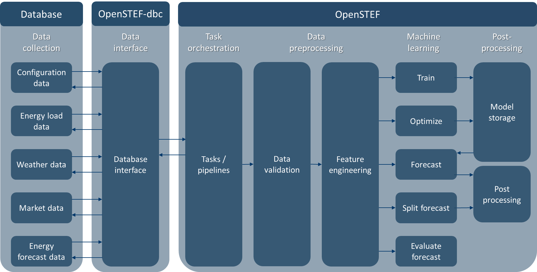
OpenSTEF is set up as a Python package that performs machine learning in order to forecast energy loads on the energy grid.

OpenSTEF contains:

• Prediction job: input configuration for a task and/or pipeline (e.g. train an XGB model for a certain location).

• Tasks: can be called to perform training, forecasting, or evaluation. All tasks use corresponding pipelines. Tasks include getting data from a database, raising task exceptions, and writing data to a database.

• Pipelines: can be called to perform training, forecasting or evaluation by giving input data to the pipeline. Users can choose to use tasks (which fetch/write data for you), or use pipelines directly (which requires fetching/writing data yourself).

• Data validation: is called by pipelines to validate data (e.g. checking for flatliners).

• Feature engineering: is called by pipelines to select required features for training/forecasting based on the configuration from the prediction job (e.g. create new features for energy load of yesterday, last week).

• Machine learning: is called by pipelines to perform training, forecasting, or evaluation based on the configuration from the prediction job (e.g. train an XGB quantile model).

• Model storage: is called by pipelines to store or fetch trained machine learning model with MLFlow (e.g. store model locally in disk/database/s3_bucket on AWS).

• Post processing: is called by pipelines to post process forecasting (e.g. combine forecast dataframe with extra configuration information from prediction job or split load forecast into solar, wind, and energy usage forecast).

• Post processing: is called by pipelines to post process forecasting (e.g. combine forecast dataframe with extra configuration information from prediction job or split load forecast into solar, wind, and energy usage forecast).

Tasks are provided in a separate Python package called openstef-dbc. If you need to use tasks, the openstef-dbc package is required in order to interface to databases for reading/writing. Currently, openstef-dbc supports interfaces for a MySQL database for configuration data (e.g. information for prediction jobs) and InfluxDB for feature data (e.g. weather, load, energy price data) and energy forecast data.

High level methodology OpenSTEF

OpenSTEF automates many typical activities in machine learning. These include the combination of input data and preparation of features. Furthermore, the train and predict methodology of OpenSTEF allows for a single-shot, multi-horizon forecast. To provide a high-level overview of these functionalities, a schematic depiction is given here.

Source file

OpenSTEF provides confidence estimates of it’s forecasts. Two methods are available. The figure below explains the differences and similarities between the two methods, as well as provide recommendations on how to the confidence estimations should be used.

Source file

Application architecture

OpenSTEF is simply a software package (i.e. a Python library). If you’re looking to run it as a full application with a graphical user interface frontend, you must deploy it with additional components.

Here are the recommended additional components if you want to run it as an application:

• Github repositories:

  • (create yourself) Data fetcher: software package to fetch input data and write it to a database (e.g. a scheduled CronJob to fetch weather data in Kubernetes).

  • (create yourself) Data API: API to provide data from a database or other source to applications and users (e.g. a REST API).

  • (create yourself) Forecaster: software package to fetch config/data and run OpenSTEF tasks/pipelines (e.g. a scheduled cron job to train/forecast in Kubernetes).

  • (open source) OpenSTEF: software package that performs machine learning to forecast energy loads on the energy grid.

  • (open source) OpenSTEF-dbc: software package that provides interface to read/write data from/to a database for openstef tasks.

• CI/CD Infrastructure

  • (create yourself) Energy forecasting Application CI/CD: Continuous Integration/Continuous Delivery pipeline to build, test, and deploy your forecasting application (e.g. to Kubernetes via Jenkins, Chef, Puppet, Tekton, etc.).

  • (open source) OpenSTEF package CI/CD: A set of GitHub Actions that build, test, and publish the OpenSTEF package to PyPI here when it is time to release a new version.

• Compute: compute resources to run your pipelines and tasks in production (e.g. on Kubernetes using any of the various providers AWS, Azure, GCP, Linode, etc.).

• Database: SQL, InfluxDB, or other database that stores fetched input data and forecasts.

• Dashboard: graphical user interface dashboard that allows uers to visualize application data (e.g. historic and forecasted energy loads)

Split forecast: Domain Adaptation for Zero Shot Learning in Sequence (DAZLS)

DAZLS is an energy splitting function in OpenSTEF. Is a technique which transfers knowledge from complete-information substations to incomplete-information substations for solar and wind power prediction. It is being used in openstef.pipeline.create_component_forecast to issue the prediction.

This function trains a splitting model on data from multiple substations with known components and uses this model to carry out a prediction for target substations with unknown components. The training data from the known substations include weather, location, and total load information of each substation and predicts the solar and the wind power of the target substations.

The model is developed as a zero-shot learning method because it has to carry out the prediction of target substations with unknown components by using training data from other substations with known components. For this purpose, the method is formulated as a 2-step approach by combining two models deployed in sequence, the Domain and the Adaptation model.

The schema bellow depicts the structure of the DAZLS model. The input of the model is data from the complete-information substations. For every known substation we have input data, source metadata and output data. At first, we feed the input data to train the Domain model. Domain model gives a predicted output. This predicted output data, linked together with the source metadata of each substation, is being used as the input to train the Adaptation model. Then, the Adaptation model provides the final output prediction of solar and wind power for the target substations.

Domain Adaptation Model

For more information about DAZLS model, see:

Teng, S.Y., van Nooten, C.C., van Doorn, J.M., Ottenbros, A., Huijbregts, M., Jansen, J.J. Improving Near Real-Time Predictions of Renewable Electricity Production at Substation Level (Submitted)

HOW TO USE: The code which loads and stores the DAZLS model is in the notebook file 05. Split net load into Components.ipynb. When running this notebook, a dazls_stored.sav file is being produced and can be used in the prediction pipeline. It is important, whenever there are changes in the dazls.py, to run again the notebook and use the newly produced dazls_stored.sav file in the repository.

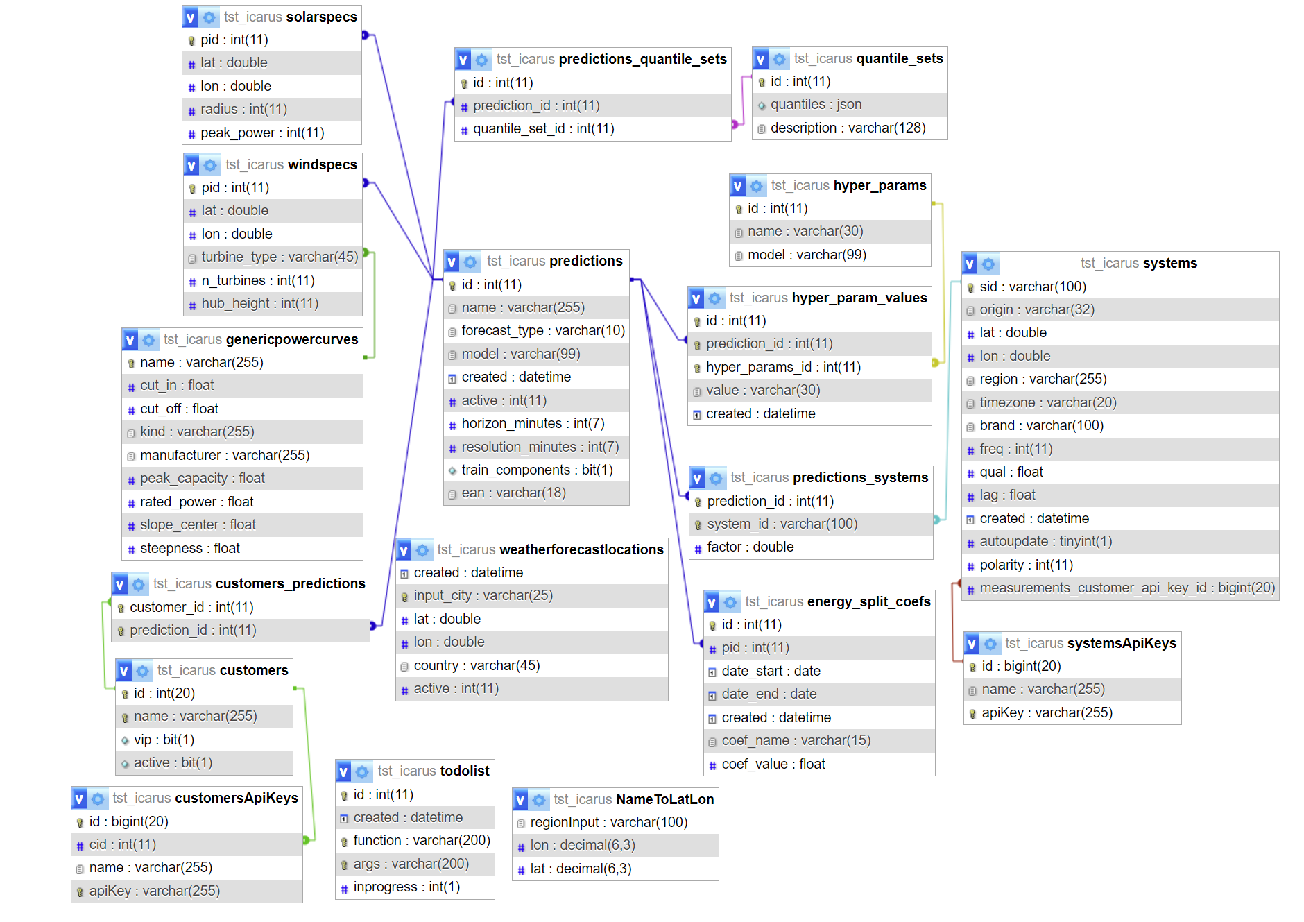
Overview of relational database

OpenSTEF uses a relational database to store information about prediction jobs and measurements. An ER diagram of this database is shown below.

The necessary tables are described in more detail bellow:

Name	Type	Comment	Example
id	int	customer id	307
name	chr	customer name	Location_A
vip	bool	extra important forecast (deprecated)	1
active	bool	activity status	1

Customer : A customer is a collection of predictions. This can be a collection of predictions belonging to a customer but also a collection of prediction belonging to a specific location or substation.

Name	Type	Comment	Example
id	int	API key id	94
cid	int	customer id	307
name	chr	customer name	Location_A
apiKey	chr	API key value	uuid-Location_A

For users to post measurements or retrieve forecasts related to a specific customer (used internally by Alliander).

customers_predictions

Correspondence table between customer ids and prediction jobs ids.

Name	Type	Comment	Example
customer_id	int	customer id	307
prediction_id	int	prediction job id	313

Contains the generic load curves of wind turbines. These curves are two-parameters sigmoids (center and slope).

Name	Type	Comment	Example
name	chr	turbine name	Vestas V112
cut_in	float	min wind speed to produce (m/s)	3
cut_off	float	max wind speed to produce (m/s)	25
kind	chr	onshore / offshore	onshore
manufacturer	chr		Enercon
peak_capacity	float	max power (W)	3040270
rated_power	float	rated power (W)	3000000
slope_center	float	Wind speed corresponding to 50% of rated power (m/s)	7.91
steepness	float	See formula	0.76

In openstef/feature_engineering/weather_features.py, the power delivered by a wind turbine is computed as

\[P(v) = \frac{P_{rated}}{1 + e^{- k(v - c)}},\]

where \(v\) is the windspeed at hub height, \(P_{rated}\) = rated_power, \(k\) = steepness and \(c\) = slope_center.

Name	Type	Comment	Example
regionInput	chr	region name	Leeuwarden
lon	decimal	longitude	5.800
lat	decimal	latitude	53.201

This table is used for looking up coordinates for specific locations that can be used directly for retrieving weather data.

Contains prediction jobs.

Name	Type	Comment	Example
id	int	prediction job id	313
name	chr	customer name	Location_A
forecast_type	chr	type of forecast	demand
model	chr	type of model	xgb
created	datetime	creation datetime of the prediction job	2019-05-16 14:53:38
active	int	0 = off; 1 = on;
horizon_minutes	int	max forecast horizon (minutes)	2880
resolution_minutes	int	time resolution of forecasts (minutes)	15
train_components	bool	Optional: Carry out energy splitting for this prediction job	1
ean	chr	EAN of the connectionpoint if the prediction corresponds to a connection point. See also: https://en.wikipedia.org/wiki/International_Article_Number	000000000000000003

Prediction: A prediction is the core concept in openSTEF and largley translate to the prediction_job in the openSTEF code. To make a prediction a prediction is usualy coupled to one or more systems. These systems provide the measurement data for which a forecast is made.

Correspondence table between prediction jobs and the set of quantiles to forecast.

Name	Type	Comment	Example
id	int		22
prediction_id	int	prediction job id	313
quantile_set_id	int	id of the quantile sets	1

Correspondence table between prediction jobs and systems.

Name	Type	Comment	Example
prediction_id	int	prediction job id	317
system_id	chr	system id	Location_A_System_1
factor	double	Optional factor to multiply before addition	-2.0

• A prediction job can correspond to multiple systems

• A system can be linked to multiple prediction jobs

• When mulitple systems are coupled to a prediction all these systems are added and the forecast is made for the sum. I ffor whatever reason a system should not be added but subtracted it is possible to set the factor to -1. Is some scaling needs to be carried out in the sum the factor can be changed from 1 (default) to the desired scaling factor.

System : Represents a physical measurement system. All metadata is saved in this SQL table, the actual timeseries can be retrieved from influx by the corresponding system id.

Contains the specifications of the quantile sets.

Name	Type	Comment	Example
id	int	quantile set id
quantiles	json	list of quantiles	[0.05, 0.1, 0.3, 0.5, 0.7, 0.9, 0.95]
description	chr		Default quantile set

Configuration for PV forecasts for each prediction job

Name	Type	Comment	Example
pid	int	prediction job id	123
lat	double	latitude	51.9850343
lon	double	longitude	5.8956792
radius	int	radius in km	10
peak_power	int	max power	1000

2 cases:

• Radius = ‘None’ : when the forecast is for a specific system

• Radius > 0 when the forecast is for a region

Contains informations about systems.

Name	Type	Comment	Example
sid	chr	system id	Location_A_System_1
origin	chr	origin of the system data	ems (energy management system = SCADA)
lat	double	latitude	5.837
lon	double	longitude	51.813
region	chr		Gelderland
timezone	chr		UTC
brand	chr	additional information on measurements	accurate_inc
freq	int	additional information on measurements	5
qual	float	additional information on measurements	1
lag	float	additional information on measurements	15
created	datetime	Date when the system is registred in openSTEF	2021-01-25 09:44:00
autoupdate	tinyint	deprecated	1
polarity	int	sign convention for production and load	-1/1
measurements_customer_api_key_id	int	API to post measurements	199

Polarity is a factor used to make the measurment comply with positive consumption and negative production of energy.

API key to retrieve systems measurements.

Name	Type	Comment	Example
id	int	API key id	199
name	chr		Measurements
apiKey	chr	API key value	uuid-Measurements

Contains the locations of the weather stations. These are used when retrieving weather data for a prediction.

Name	Type	Comment	Example
created	datetime		2023-06-08 18:26:44
input_city	chr		Deelen
lat	double		52.067
lon	double		5.8
country	chr		NL
active	int		1

This table is empty in openstef-reference. Contains the information for the wind power forecast related to a prediction job.

Name	Type	Comment	Example
pid	int	prediction job id
lat	double
lon	double
turbine_type	chr	corresponds to the field ‘name’ in genericpowercurves
n_turbines	int	number of wind turbines
hub_height	int	height of the turbines (m)

The hub height is used to extrapolate the wind speed forecast at the correct height.

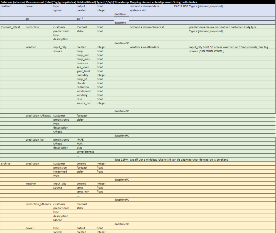
Overview of timeseries database schema

OpenSTEF uses a timeseries database to store all timeseries data. A diagram of its structure is shown bellow.