

Forecasting Quickstart#
Train a GBLinear model on real energy data and generate probabilistic forecasts with confidence intervals — all in under a minute.
What you’ll learn:
Load the Liander 2024 benchmark dataset
Configure a forecasting workflow with
ForecastingWorkflowConfigTrain a model and inspect evaluation metrics
Generate quantile forecasts (P10 / P50 / P90)
Visualize predictions against actuals
Note
This tutorial uses a small data slice for fast execution.
See examples/benchmarks/ for production-scale runs.
Key API references:
ForecastingWorkflowConfig
create_forecasting_workflow
· LeadTime
· Q
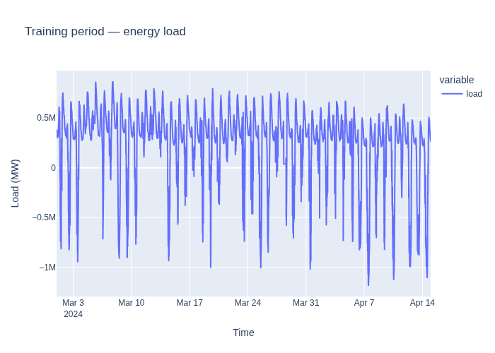
Load the dataset#
The Liander 2024 benchmark dataset contains load measurements, versioned weather forecasts, EPEX prices, and load profiles for a medium-voltage feeder in the Netherlands.
We split the data into:
45 days of training data
7 days for forecasting
The predict window includes 14 days of history before the forecast start so
that lag features (e.g. load_lag_P7D) can be computed during prediction.
from datetime import datetime, timedelta

from openstef_core.testing import load_liander_dataset

dataset = load_liander_dataset()

train_start = datetime.fromisoformat("2024-03-01T00:00:00Z")
train_end = train_start + timedelta(days=45)
forecast_end = train_end + timedelta(days=7)

train_dataset = dataset.filter_by_range(start=train_start, end=train_end)

# Include 14 days of history before forecast start for lag feature computation
predict_dataset = dataset.filter_by_range(
    start=train_end - timedelta(days=14),
    end=forecast_end,
)

print(
    f"Training:  {train_dataset.data.shape[0]:,} rows, "
    f"{train_dataset.data.index.min():%Y-%m-%d} to {train_dataset.data.index.max():%Y-%m-%d}"
)
print(
    f"Predict:   {predict_dataset.data.shape[0]:,} rows, "
    f"{predict_dataset.data.index.min():%Y-%m-%d} to {predict_dataset.data.index.max():%Y-%m-%d}"
)
Training:  4,320 rows, 2024-03-01 to 2024-04-14
Predict:   2,016 rows, 2024-04-01 to 2024-04-21
Configure the workflow#
ForecastingWorkflowConfig bundles all settings — model type, horizons, quantiles,
and feature columns — into a single object. create_forecasting_workflow turns
it into a ready-to-use pipeline with preprocessing, training, and postprocessing.
We pick GBLinear (gradient-boosted linear model) for its speed and ability to extrapolate beyond training data.
from openstef_core.types import LeadTime, Q
from openstef_models.presets import ForecastingWorkflowConfig, create_forecasting_workflow
from openstef_models.presets.forecasting_workflow import GBLinearForecaster

workflow = create_forecasting_workflow(
    config=ForecastingWorkflowConfig(
        model_id="quickstart_gblinear",
        model="gblinear",
        horizons=[LeadTime.from_string("PT36H")],
        quantiles=[Q(0.5), Q(0.1), Q(0.9)],
        target_column="load",
        # Weather features available in the Liander dataset
        temperature_column="temperature_2m",
        relative_humidity_column="relative_humidity_2m",
        wind_speed_column="wind_speed_10m",
        radiation_column="shortwave_radiation",
        pressure_column="surface_pressure",
        verbosity=0,
        mlflow_storage=None,
        gblinear_hyperparams=GBLinearForecaster.HyperParams(n_steps=50),
    )
)
Train the model#
workflow.fit() runs the full pipeline: feature engineering, data validation,
model training, and evaluation on a held-out test split.
result = workflow.fit(train_dataset)

if result is not None:
    print("Training metrics:")
    print(result.metrics_full.to_dataframe())

    if result.metrics_test is not None:
        print("\nTest-set metrics:")
        print(result.metrics_test.to_dataframe())
Training metrics:
   quantile        R2  observed_probability
0       0.5  0.809093              0.465509
1       0.1  0.502659              0.083565
2       0.9  0.471458              0.907639
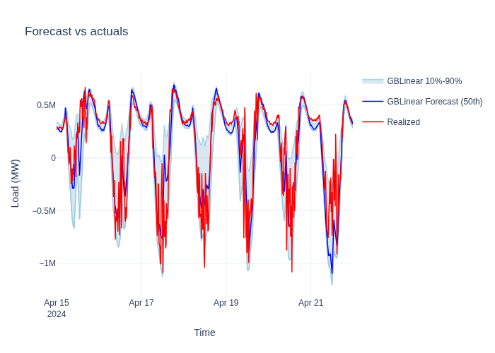
Generate forecasts#
The trained workflow produces a ForecastDataset with point predictions and
quantile bands. The P10-P90 interval covers 80 % of expected outcomes.
To improve the reliability of these quantile estimates, see
Quantile Calibration.
from openstef_core.datasets import ForecastDataset

forecast: ForecastDataset = workflow.predict(predict_dataset, forecast_start=train_end)

print(f"Forecast rows: {len(forecast.data)}")
print(f"Quantiles:     {forecast.quantiles}")
forecast.data.tail()
Forecast rows: 672
Quantiles:     [0.5, 0.1, 0.9]
| quantile_P50 | quantile_P10 | quantile_P90 | load | stdev | |
|---|---|---|---|---|---|
| timestamp | |||||
| 2024-04-21 22:45:00+00:00 | 371693.81250 | 320575.90625 | 387800.78125 | 353333.333333 | 37672.244870 |
| 2024-04-21 23:00:00+00:00 | 359203.81250 | 301154.53125 | 381089.50000 | 336666.666667 | 34140.093713 |
| 2024-04-21 23:15:00+00:00 | 346523.37500 | 296382.65625 | 373214.93750 | 323333.333333 | 34140.093713 |
| 2024-04-21 23:30:00+00:00 | 333368.59375 | 288091.50000 | 364443.81250 | 323333.333333 | 34140.093713 |
| 2024-04-21 23:45:00+00:00 | 321874.68750 | 282207.59375 | 356208.00000 | 316666.666667 | 34140.093713 |
Visualize the results#
ForecastTimeSeriesPlotter overlays measurements and predictions with shaded
confidence bands in a single interactive chart.
Next steps#
Backtesting Quickstart — evaluate how this model performs on historical data with realistic temporal constraints.
Building a Custom Pipeline — build a model from individual transforms when presets don’t cover your use case.